Insert a picture onto the sheet
See also: “How to set a password to protect a file in Excel: workbook, sheet”
First, we carry out the preparatory work, namely, open the required document and go to the required sheet. Next we proceed according to the following plan:
- We stand in the cell where we plan to insert the picture. Switch to the “Insert” tab, where we click on the “Illustrations” button. In the drop-down list, select “Drawings”.
- A window will appear on the screen in which you need to select the desired picture. To do this, first go to the folder containing the required file (the “Images” folder is selected by default), then click on it and click the “Open” button (or you can simply double-click on the file).
- As a result, the selected picture will be inserted onto the book sheet. However, as you can see, it is simply placed on top of the cells and is in no way connected with them. Therefore, we move on to the next steps.
Setting up the picture
Now we need to customize the inserted image by giving it the required dimensions.
- Right-click on the picture. In the list that opens, select “Size and properties”.
- A picture format window will appear, where we can configure its parameters in detail:
- dimensions (height and width);
- angle of rotation;
- height and width in percentage;
- maintaining proportions, etc..
- However, in most cases, instead of going to the picture format window, the settings that can be made in the “Format” tab are sufficient (in this case, the picture itself should be selected).
- Let's say we need to adjust the size of the picture so that it does not extend beyond the boundaries of the selected cell. You can do this in different ways:
- go to the “Dimensions and Properties” parameters through the context menu of the image and adjust the size in the window that appears.
- set the dimensions using the appropriate tools in the “Format” tab on the program ribbon.
- Holding down the left mouse button, drag the lower right corner of the picture diagonally upward.
How to insert pictures into Excel
Hello friends. I think each of you wants to know how to insert pictures into Excel. Indeed, often images on an Excel sheet provide important additional information. For example, a photo of a product, a location map, a supplier’s logo, etc.
To insert an image from your computer’s hard drive , execute the ribbon command: Insert – Illustrations – Drawings. An explorer window will open, in which find and select the desired file, click “insert”. The picture will immediately appear on the active sheet.
In some cases, it is convenient to insert a picture from the Internet . On the ribbon, perform Insert – Illustrations – Images from the Internet.
The program allows you to download pictures from the OneDrive cloud service, connected social network accounts, or find the desired image using the Bing search engine. Select the appropriate option, check the boxes for the uploaded images and click “Insert”. The pictures will be downloaded from the source and appear on the sheet.
When you insert an image from a Bing search, you will be politely reminded to respect copyright.
You can also paste an image by copying. If there is an image in any of the open applications, copy it (for example, by pressing Ctrl+C). Return to Excel and press Ctr+V, the picture will be inserted.
The new generation of Microsoft Excel has introduced an interesting feature - inserting a copy of the screen. For example, you need to add a screenshot of some of your development. Open the desired window, then go to Excel and click Insert - Illustrations - Take Screenshot. Excel will display thumbnails of all open windows, select the one you need. A copy of this window will immediately appear on the sheet.
And starting with Excel 2013, you can paste only the part of the window you need. To do this, select Insert – Illustrations – Take Screenshot – Screen Clipping. The program will display the inserted window with a cropping frame. After selecting the desired area, the picture will appear on the sheet.
Once you have inserted the drawing onto the sheet, you can embellish it a little. Click on it to highlight it. A new tab will appear on the ribbon: Working with Pictures – Format.
The first thing you can do is change the style. The program will offer you several ready-made drawing design layouts. The drop-down list of styles is located in the “Picture Styles” block.
If none of them suits you, set your own using the “Picture Border”, “Picture Effects”, “Picture Layout” ribbon buttons. If you use the Graphic Layout options, it will be converted to a SmartArt object and two more tabs will appear on the ribbon to customize it.
You will find an excellent set of tools for formatting pictures on the ribbon Working with Pictures – Format – Change. Here you can remove the background from the picture, apply artistic filters, make corrections and adjust color tones. The functionality is comparable to some graphic editors. In addition, everything is done very simply and intuitively.
A very useful option in this group is “ Compress Picture ”. The program optimizes drawings to reduce file size and speed up loading.
As with other graphic objects (shapes, SmartArt, WordArt), there is a group of Arrange commands. These commands will help you align inserted images vertically and horizontally, distribute them evenly, rotate them, group and ungroup them.
In the “Size” block, specify the exact dimensions of the picture, if necessary.
Well, to “fine-tune” all possible parameters of an object, click on it and press Ctrl+1. The dialog box that opens will contain a complete list of all image settings: color, outline, text format, shadows, brightness, contrast, print resolution, cell binding and much more. A description of all the settings would take and make the article several times longer, so I’ll leave them for you to study on your own.
Perhaps that's all on this topic. From Excel graphical objects, we just need to study the equation editor. If you are a student or a teacher of exact sciences, do not miss this short post, it is just for you! See you again!
Attaching a picture to a cell
So, we inserted a picture into an Excel sheet and adjusted its size, which allowed it to fit within the boundaries of the selected cell. Now you need to attach the picture to this cell. This is done so that in cases where a change in the table structure leads to a change in the original location of the cell, the picture moves with it. You can implement this as follows:
- Insert an image and adjust its dimensions to fit the cell borders, as described above.
- Click on the picture and select “Size and properties” from the list that opens.
- The already familiar picture format window will appear in front of us. After making sure that the dimensions correspond to the desired values, and also that the “Maintain proportions” and “Relative to original size” checkboxes are checked, go to “Properties”.
- In the drawing properties, check the boxes next to the “Protectable object” and “Print object” items. Also, select the option “Move and resize with cells”.
Protecting a cell with an image from changes
This measure, as the title suggests, is needed to protect the cell with the picture it contains from being changed or deleted. Here's what you need to do for this:
- We select the entire sheet, for which we first deselect the image by clicking on any other cell, and then press the key combination Ctrl+A. Then call the context menu of cells by right-clicking anywhere in the selected area and selecting “Format Cells”.
- In the formatting window, switch to the “Protection” tab, where we uncheck the box next to “Protected cell” and click OK.
- Now click on the cell where the picture was inserted. After that, also through the context menu, go to its format, then go to the “Protection” tab. Check the box next to the “Protected cell” option and click OK.
Note: if a picture inserted into a cell completely overlaps it, then clicking the mouse buttons on it will call up the properties and settings of the picture. Therefore, to go to a cell with an image (select it), it is best to click on any other cell next to it, and then, using the navigation keys on the keyboard (up, down, right, left), go to the required one. Also, to call the context menu, you can use a special key on the keyboard, which is located to the left of Ctrl.
- Switch to the “Review” tab, where we click on the “Protect Sheet” button (when the window size is compressed, you first need to click the “Protection” button, after which the desired item will appear in the drop-down list).
- A small window will appear where we can set a password to protect the sheet and a list of actions that users can perform. When ready, click OK.
- In the next window, confirm the entered password and click OK.
- As a result of the actions performed, the cell in which the picture is located will be protected from any changes, incl. removal.
At the same time, the remaining cells of the sheet remain editable, and the degree of freedom of action in relation to them depends on which items we selected when enabling sheet protection.
Attaching an image
If you simply insert a picture, it will not move in cases where the location of the cells changes. In some cases it is desirable to avoid this. For example, if a page contains a list of company employees, and their photographs are inserted opposite, then it is convenient when, as a result of sorting, the arrangement of the data is preserved .
Linking a picture to a cell in Excel can be done using several methods, which will be discussed below.
Sheet protection
To do this you need to do the following:
- It is necessary to expand the boundaries of the cell and change the size of the picture so that the image fits inside the cell.
- You need to right-click on the picture and select the line “ Size and properties ” in the context menu.
- On the left side of the window that opens we find a list of tabs. You need to go to " Size ".
- You need to make sure that the entire picture fits inside the cell. The two available checkboxes (“ Relative to size ” and “ Maintain proportions ”) should be checked.
- Next, you need to go to the “ Properties ” tab. In the top switch, select the line corresponding to the fact that the object will move along with the corresponding cells. Check both checkboxes (“ Protected object ” and “ Print ”).
- Now you need to select the entire page . This is done by pressing the key combination “ Ctrl+A ”. Then we move on to formatting the cell. To do this, you need to right-click on it.
- You must select the cell in which the image is located. On the “ Protection ” tab, you should mark the line where we are talking about protecting cells.
- Now in the main menu in the “ Review ” tab you need to select the line “ Sheet protection ”. On the screen that opens, you need to enter a password to unlock and confirm the entry.
It is important to consider that you need to install protection both on the desired cell and on the entire page. After this, the image becomes linked to the corresponding cell.
Inserting a note
As you know, Excel has the ability to set a note to a specific cell. You can use it to attach a drawing.
Insert a picture into a cell note
In addition to inserting a picture into a table cell, you can add it to a note. We will describe how this is done below:
- Right-click on the cell where we want to insert the picture. In the drop-down list, select the “Insert Note” command.
- A small area will appear for you to enter your note. Place the cursor over the border of the note area, right-click on it and in the list that opens, click on the “Note Format” item.
- The note settings window will appear on the screen. Switch to the “Colors and Lines” tab. In the fill options, click on the current color. A list will open in which we select the “Fill methods” item.
- In the fill methods window, switch to the “Drawing” tab, where we click the button with the same name.
- An image insertion window will appear, in which we select the “From file” option.
- After this, a picture selection window will open, which we already encountered at the beginning of our article. Go to the folder containing the file with the desired image, and then click the “Insert” button.
- The program will return us to the previous window for selecting fill methods with the selected pattern. Check the box for “Maintain picture proportions” and then click OK.
- After this, we will find ourselves in the main note format window, where we switch to the “Protection” tab. Here we uncheck the box next to the “Protected object” item.
- Next, go to the “Properties” tab. Select the option “Move and change the object along with the cells.” All settings are completed, so you can click OK.
- As a result of the actions performed, we were able to not only insert a picture as a note to the cell, but also link it to the cell.
- If desired, the note can be hidden. In this case, it will only be displayed when you hover over the cell. To do this, right-click on the cell with the note and select “Hide Note” from the context menu.
If necessary, the note is included back in the same way.
Inserting into a cell
Before you insert a picture into a cell in Excel, you need to prepare the image. It must be located on a computer from where it can be downloaded into an electronic document.
Before you can insert a picture into a cell, you need to start Excel . Then select the cell that is located in the place where you want to place the drawing. In the “ Insert ” tab, click on the “ Drawing ” button. This will open a screen for you to select the desired file. You need to find the directory where the image is stored and point to it. After confirmation, you can see the picture placed on the Excel page in the right place.
Insert the image using developer mode
See also: “Break-even point in Excel: calculation, chart”
Excel also provides the ability to insert a picture into a cell through the so-called Developer Mode. But first you need to activate it, since it is turned off by default.
- Go to the “File” menu, where we click on the “Options” item.
- A settings window will open, where in the list on the left, click on the “Customize Ribbon” section. After that, in the right side of the window in the ribbon settings, find the line “Developer”, check the box next to it and click OK.
- We go to the cell where we want to insert the image, and then go to the “Developer” tab. In the “Controls” tool section, find the “Insert” button and click on it. In the list that opens, click on the “Image” icon in the “ActiveX Elements” group.
- The cursor will change to a cross. Using the left mouse button held down, select the area for the future image. If necessary, the dimensions of this area can then be adjusted or the location of the resulting rectangle (square) can be changed to fit it inside the cell.
- Right-click on the resulting figure. In the list of commands that opens, select “Properties”.
- A window with the properties of the element will appear in front of us:
- in the value of the “Placement” parameter, indicate the number “1” (the initial value is “2”).
- in the area for entering the value opposite the “Picture” parameter, click on the button with an ellipsis.
- An image upload window will appear. Select the desired file here and open it by clicking the appropriate button (it is recommended to select the “All Files” file type, since otherwise some of the extensions will not be visible in this window).
- As you can see, the picture is inserted onto the sheet, however, only part of it is displayed, so adjusting the dimensions is required. To do this, click on the small downward triangle icon in the “PictureSizeMode” parameter value field.
- In the drop-down list, select the option with the number “1” at the beginning.
- Now the entire image fits inside the rectangular area, so the settings can be closed.
- All that remains is to attach the image to the cell. To do this, go to the “Page Layout” tab, where we click the “Organize” button. In the drop-down list, select “Align”, then “Snap to grid”.
- Done, the picture is attached to the selected cell. In addition, now its borders will “stick” to the borders of the cell if we move the picture or change its size.
- This will allow you to accurately fit the design into the cell without much effort.