It is difficult to imagine the work of an Internet marketer without spreadsheets. Previously, the main tool was Excel from MS Office, but now more and more specialists are switching to Google Sheets. And they can be understood:
- Google's online service is free.
- Collaboration is conveniently implemented - no need to send files to each other a thousand times.
- Changes are saved automatically.
- There is a version history - if necessary, you can roll back to the moment from which everything went wrong.
- You can set up automatic import of data from third-party sources - analytics services, advertising offices, call tracking, etc.
Google Sheets is a very versatile and functional tool with a lot of features and use cases. Using formulas alone, you can write a separate book. In order not to turn the material into a monstrous longread that no one will even read to the middle, I will not consider advanced features, such as working with scripts, go into small details and provide lengthy instructions for each function.
This guide will show you what you can do in Google Sheets, help you find ways to use it in your work, and understand what direction to dig in to learn how to work effectively in the program.
Getting started with Google Sheets
You can create new tables and open previously created ones on the main page of the service and through Google Drive.
The main Google Sheets displays all the sheets you've ever opened. By default they are sorted by viewing date. To open an existing table, click on it once. A new file can be created by clicking the plus in the lower right corner.
From Google Drive, tables can be opened by double clicking. To create a new file, click “Create” in the upper left corner or call the context menu with a right click. Here you can also start working with a blank table or choose one of Google's templates.
The Ultimate Guide to Google Docs: Everything You Didn't Know But Were Afraid to Ask
There is no need to save tables - everything is automatically saved to Google Drive as you work. Once you're done, you can simply close the file—no data will be lost. By default, files created through the Google Sheets service are saved in the root of Drive. To move it to a folder, click on the icon next to the table name and select a destination. Before you can move the newly created table, you must rename it.
You can also transfer files to Google Drive using drag&drop or by right-clicking on it and selecting “Move to...”.
How to open an Excel file in Google Sheets
Google Sheets supports Excel tables. You can open such a file in the service in two ways:
- Upload the file to Google Drive using the Create button and open it like a regular Google spreadsheet.
- While in any table, go to the "File" menu and select "Open" or use the combination Ctrl + O. In the window that opens, go to the "Load" tab.
This also works in the opposite direction - Google Sheets files are downloaded to your computer in formats that Excel supports: XLSX and CSV. To do this, go to the “File” → “Download As” menu and select the format. You can also save the table in ODT format to open it in Open Office.
Complex tables with many formulas, graphs and charts may not open correctly when transferred to another format. Once you've uploaded the file to Google Sheets or downloaded it to Excel, check that everything is displayed and working correctly.
Google Sheets Toolbar
In Google, these elements look simpler than in Excel. However, if you are used to working with MS Office software, it will take some time to get used to it.
Let's briefly go through the tools on the panel. We will talk about some of them in more detail later, in the appropriate sections.
Like Excel, the toolbar in Google Sheets is divided into blocks:
- Undo and redo the last action, print the document, copy formatting. The last tool is convenient to use when you need to apply the same formatting to several cells. Select a cell, click on the tool in the panel, and then click on the cell that you want to format.
- Change scale. Makes the table larger or smaller, range from 50 to 200%.
- Change the data format in cells - select monetary or percentage, increase and decrease the number of decimal places in a numeric one, select other formats in the drop-down menu.
- Font.
- Font size.
- Text formatting - style, text and background color.
- Cell formatting - color filling, borders, merging.
- Text alignment - horizontally, vertically, translation and rotation settings.
- Other tools:
- add link;
- Add a comment;
- insert chart;
- create a filter;
- use functions.
- Display the sheet and input direction.
- Input method - here you can enable the on-screen keyboard and handwriting input field.
- Hide menu - by clicking on the arrow on the right, the main menu, along with the table header, access settings and account icon, is removed. All that remains is the toolbar.
At the bottom there is a panel for switching between sheets and operations with them. To create a new page in the current file, click “+” in the lower left corner. By clicking on the arrow next to the sheet title, a menu will open where you can rename, delete, move, copy and hide the sheet, as well as protect it from editing and change the color of the label.
The hidden sheet shortcut will not appear in the general panel. To view and return it, go to the menu “View” → “Hidden Sheets” and find the one you need in the list.
Operations with cells, rows and columns
Table elements - rows, columns and cells - can be added, deleted and hidden through the "Edit" menu or the context menu, which opens by right-clicking on the selected element. For some actions, you need to choose what will happen to surrounding elements after deletion or insertion - where the data, rows and columns will move.
How to freeze lines
When working with large amounts of data, it is useful to always keep the row and column headings in front of you. To do this, they can be fixed. Place the cursor in a cell of the desired row or column, open the menu “View” → “Freeze” and select one of the options.
How to move table elements
Rows, columns, and cells in Google Sheets can be rearranged and moved around the entire sheet.
To move a row or column, select it by clicking on the header, open the Edit menu and select Move Row/Column left, right, up or down.
In addition, rows, columns and cells can be moved simply by dragging and dropping. To do this, move the cursor over the edge of the selected element so that it looks like a “hand”, grab the element with a left click and drag it to the desired location without releasing the mouse button.
History of changes in Google Sheets
Google Sheets automatically saves not only the current version, but also the entire history of changes. To open it, click on the line “All changes are saved to Disk” to the right of the Main Menu.
In history mode, you cannot edit the table, but on the right you can select, view and, if desired, restore any of the previous versions.
It happens that it is impossible to restore the previous version - this is not your table and you did not edit it. If you click Restore, any changes the other person made after a certain point will be deleted. Working with the previous version in history mode is also difficult - it’s impossible to even properly select and copy data, let alone use filters and formulas. In this case, Google Sheets has the ability to copy an earlier version.
By clicking, the program will create a copy of the table in the form you need.
Sharing
One of the undeniable advantages of Google Sheets over Excel is the ability to collaborate. To share your file with colleagues, click the blue “Sharing Settings” button in the upper right corner and set the settings.
You can give access to the file to individual users, those with a link, or the entire Internet. There are also different levels: “Editing”, “Commenting”, “Viewing”.
Life hack: if you link to other people’s sites in your tables and don’t want the contents of the file to be seen by others, do not share the link. Owners of sites that you link to can get a link to the file from referral sources reports and open it.
How to delete and restore a table
To delete a Google Sheet, open the File menu and select Delete.
You can delete tables in the Google Drive interface and on the main page of the Google Sheets service without opening them. In the first case, select the unnecessary file and click the trash can icon on the top panel; in the second, open the file menu and find the “Delete” item.
Open Google Sheets
Let's start by defining what exactly the average user means when they ask the question: “How do I open my Google Sheets?” Surely, this means not only the banal opening of a file with a table, but also opening it for viewing by other users, that is, providing shared access, which is often necessary when organizing collaboration with documents. Next, we will talk about solving these two problems on a computer and mobile devices, since Tables are presented both as a website and as applications.
Note: All table files created by you in the application of the same name or opened through its interface are saved by default on Google Drive - the company's cloud storage, which includes the Documents application package. That is, by logging into your Drive account, you can also see your own projects and open them for viewing and editing.
Working with data in Google Sheets
How to Edit Google Sheets
Data in the table can be entered from the keyboard, added via “copy” → “paste” and imported from various sources.
To enter data into a table, simply place the cursor on a cell and start typing. You can move around the sheet using the mouse, arrows and hotkeys - more about them at the end of the article. To edit data in a cell, double-click on it, press Enter, or place the cursor in the desired place in the formula bar.
How to protect data from editing
You can prevent colleagues from editing data in the entire table, on individual sheets, ranges, and even cells. The prohibition of editing the entire table is configured through access levels, and there is a separate tool for cells and ranges.
Call the context menu by right-clicking and select “Protect Range” or open the “Data” menu and click “Protected Sheets and Ranges”. In the form that opens on the right, click “Add sheet or range.” Enter a description. If you want to close a range from editing, click the table icon on the corresponding tab and select the desired cells on the sheet. To protect an entire sheet, go to another tab and select it from the list. Click "Set Permissions" and configure access.
You can specify a limited list of users who have the right to edit specified sheets and cells, or limit yourself to a warning. In the latter case, when you try to edit a protected range, the program will display a warning message.
Comments and notes
In Google Sheets, you can mark cells with comments and notes. Cells with comments are highlighted with a black triangle in the upper right corner, and cells with comments are highlighted with a yellow triangle. The main difference is that a comment can be replied to by other users, but a note cannot.
Comments can be closed by clicking “Issue resolved”, a note can only be deleted through the “Edit” menu, or by calling the context menu with a right click.
To add a note, select the desired cell, right-click and find the “Insert Note” option. There is also the “Insert Comment” function, but using the icon on the toolbar will be faster.
Data formats
Data—The text and numbers you enter into a table can be displayed in different formats. There are several dozen options for presenting data, but all of them can be reduced to 7 main ones:
- text;
- number;
- percent;
- finance;
- currency;
- date of;
- time.
All other formats are derivatives of the main ones. The currency can be displayed with tenths or rounded to whole numbers, replace “r.” before figures for other currencies. The date is displayed as "12/2/2018" or "Sunday, December 2, 2018" - and in ten different variations. The same goes for other formats.
To change the format of data in a cell, row, column, or range, select it, choose Format → Numbers, and choose the one you want.
Frequently used ones are listed in the “Numbers” section, the rest are hidden in the “Other formats” section.
Conditional data formatting
In Google Sheets, you can change the appearance of text and cells - font, size, style, font and fill color, alignment, border color and style, text wrapping rules. All the necessary tools are located on the panel above the work area, which we talked about above.
Sometimes you want the formatting of cells to change automatically depending on what data is in them. To do this, Google Sheets uses conditional formatting rules. They can be set for the entire table, a single range, a row, a column, or even a single cell.
To set up rules, go to Format → Conditional Formatting. A dialog box will appear on the right. By clicking on “Add Rule” the settings will open. Depending on the task, you can set up a rule by which cells will be repainted in one color, or create a gradient. The rule for formatting cells with one color is configured in 3 steps:
- Please enter a range.
- Set formatting conditions.
- Customize the format - text color and style, cell fill.
There are a total of 18 formatting conditions in Google Sheets for text data, numbers and dates. So, you can select cells that contain any data, certain words, numbers less than a specified value, etc.
To create more complex rules, you need to select the “Your formula” condition and use functions. This topic deserves a separate large article, so we won’t dwell on it here. Let's look at an example of using standard conditions.
You conduct contextual advertising and upload indicators to tables to analyze performance. To identify underperforming ads, you need to look for lines with a CTR of less than 1%. Create a rule for the corresponding column, according to which cells with a value less than one will be highlighted in color.
The gradient is useful when you need, for example, to visualize the deviation of data up and down from the optimal value.
Filters and sorting
Tools for sorting, filtering, checking and grouping table contents are located in the “Data” item of the main menu.
Sorting. At the top of the drop-down list there are buttons for quickly sorting the sheet in forward or reverse alphabetical order by the column with the selected cell. Numeric values are sorted from smallest to largest and vice versa, respectively.
If the table has a header row, quick sort will move them too. To keep them in place, choose Range Sort from the Data menu. It will become active when you select the desired range. By clicking, a dialog box will open with a choice of column and sort order - forward or reverse. To keep the header row in place, check the box next to “Data with header row.”
Filters hide data from the table that is not currently needed. This is convenient when you work with large arrays - look at publications on a separate platform or type of content in a large content plan, analyze data on achieving one goal in an analytical report.
The Data menu has two tools for filtering table contents: “Create Filter” and “Filters...” If one user filters table contents using the first tool, others will also have theirs sorted. Therefore, if you need to hide part of the data only for yourself, so as not to disturb your colleagues, select “Data” → “Filters...” → “Create a new filter.”
By clicking, the filtering mode will turn on - all the settings you make will be saved. You can create several filtering modes, all of which will appear in the “Filters...” drop-down menu. To make them easier to navigate, give each a clear name. The default names are "Filter 1", "Filter 2", etc.
Lifehack: If you want to show another user the data in the form in which you filtered it using the filtering mode, just turn it on and send the copied link.
In tables with View Only access mode, the Create Filter function is inactive. To display the data the way you want, select Data → Filters... → Create a new temporary filter.
Data checking
The tool checks whether the data in the cell matches the specified parameters. For example, one column should only contain dates. To check if there are any errors, select “Data Check” from the “Data” menu and set the settings:
- Range of cells → click on the field and select the desired column.
- Rules → select “Date” from the drop-down list, then “is a valid date”
- Click "Save".
Red marks will appear in the upper right corner of cells with incorrect data, and when you hover over them, a window with explanations will appear.
If the data in the range being checked is edited frequently, you can prevent errors in the future. In the “For invalid data” section, select “prevent data entry,” and when someone tries to enter something other than a valid date in the column, the system will display a warning and prevent you from editing the cell. By default, the service displays standard warning text, but you can set your own. To do this, check the box next to “Show help text for data verification” in the settings and enter your option in the field.
In addition to matching the data to the date format, you can set dozens of different rules for numeric, text, and other data. For example, you can verify that numbers in a range are less than, greater than, or equal to a certain value. As in the case of conditional formatting, the data verification function, in addition to the rules provided by the system, supports entering its own formulas.
Pivot tables
Pivot tables are a popular data analysis tool. It comes in handy when you need to structure and visualize large amounts of information to make it easier to draw conclusions.
Let me give you an example. You conduct end-to-end analytics for a beauty salon - you scrupulously record all data on orders down to the advertising source from which the lead came. Over the course of a year, a long table with thousands of rows is obtained. Task: find out which channel brought in the most profit over the past year in order to competently redistribute the advertising budget. With the help of pivot tables, we will get a simple and visual report in just a couple of clicks.
To create such a report, select the source table, go to the “Data” menu and select “Pivot Table”. The program will create a new blank sheet and open the editor on the right. In the row section, click “Add” and select the column with advertising channels. In the "Values" section, add a column with the profit data for each order. The program will sum up the profits for each channel and put them in a table. If you select the “Services” option in the “Columns” section, the table will show how much profit each channel generated for each service. You can also filter data by any column from the source table, for example, hide data for a particular service from the pivot table. To do this, you need to add the “Services” column to the “Filters” section, open the list and uncheck those services for which we do not want to take into account data.
We focus on omnichannel – we engage in comprehensive business promotion on the Internet. More details
Charts and graphs in Google Sheets
For data visualization, there are more functional and convenient tools - Google Data Studio, Power BI and others. However, sometimes it is useful to add a chart or graph directly to the table to visualize the data.
Let's look at the process of creating charts and setting up this tool using the example of a pivot table that we made in the previous paragraph. Go to the desired tab, go to the “Insert” menu and select “Diagram”. By default, the program creates a graph like this. On the right, instead of the “Pivot Table Editor”, the “Chart Editor” will open.
The visual representation included the line “Total” - the amount of profit across all channels. Since its value is several times greater than for each channel separately, the remaining columns of the diagram look too small in the background - it is inconvenient to analyze and compare. Therefore, first, let’s remove this line from the chart by editing the range - click on the table icon in the “Data range” line of the “Chart Editor” and select the desired one.
Let's see what else we can do with the diagram:
- Change type. Google Sheets supports graphs, columns, lines, scatters, pie, trees, geographic, waterfall, radar, and several other types of charts. For an explanation of which tasks specific types are best suited for, see the Google Sheets help.
- Change the accumulation type - standard or normalized. This option is useful when you display data based on multiple criteria in one chart column. It is not active for all chart types.
- Change the range of values.
- Add, remove and change axes and parameters.
Basic manipulations with the chart are collected on the “Data” tab. On the “Additional” tab you can change the appearance of the chart:
- recolor columns, lines, segments in one or different colors;
- change the font, color, style of individual elements or the entire text;
- change chart background;
- edit the title of the chart and axes, etc.
There are many settings, but they are all intuitive.
Charts created in Google Sheets can be saved as an image and published on the site by embedding the code into the page. To do this, open the drop-down menu in the upper right corner of the diagram and select the appropriate items.
Programs for creating tables, additional list
In addition to the three programs given in this review, you can focus your attention on others. More programs for creating tables:
SmartDraw. A website that you can use for work (www.smartdraw.com). The program is paid if you download it for Windows. The utility costs $10 per month. You can use it for free too. To do this, you need to register in this system online (Figure 5).
You can create tables right away on the Internet.
Edraw Max. Costs $179. The program creates various tables, maps, graphs, and so on. The created files can be saved in the following formats - Phg, Jpeg, Pdf and others.
Canva Charts. The price of this program is pleasantly surprising. It's completely free. Has the ability to save spreadsheets in regular image format. With its help, you can only edit the created table and then save it on your computer.
These programs work efficiently and create spreadsheets. So you can safely use them.
Working with functions
In Google Sheets, just like in Excel, there are functions - formulas that process data in the table - sum, compare, check for compliance with conditions, etc.
All functions are introduced according to the same principle:
- We enter the “=” sign so that the program understands what we want from it.
- Then we start entering the name of the function. The system will display a list of prompts from which you can select the one you need.
- In parentheses we indicate the data that needs to be used for calculations, and enter additional arguments if necessary.
Data for calculations can be entered manually using the keyboard or you can specify links to cells and ranges from which they need to be taken. You can also enter names for named ranges, but you must first create them. This is useful when you frequently use the same data ranges in calculations. To create a named range, go to the “Data” menu or right-click the context menu and select the appropriate item. The Named Range Editor will open on the right. Click “+Add range” and enter a name. If you haven't selected the cells you need before, click on the table icon and do so, then click "Done".
Let's look at the example of a simple function that is often used by SEOs and contextual advertising specialists - DLTR - calculates the length of a line.
We won’t describe each function in detail - there are about 400 of them. Let’s just say that using formulas here you can do everything the same as in Excel. Of course, there are formulas there that are not in the Google service, and vice versa, but there are not many of them. For example, Excel does not have the GOOGLETRANSLATE function, which translates text from one language to another.
We have already written about the functions of MS Office spreadsheets that are useful for Internet marketers; they all work perfectly in the Google service. The principle of operation of these functions is the same, but the syntax may differ. A list of all Google Sheets formulas with descriptions and syntax is in the reference book.
Excel program, functions of this program
Hello, friends! Let's look at the Excel program and its main functions. This program is included in the Microsoft Office package, which means the program itself is paid. Of course, on the Internet
You can download and install the free version of this program. But it is not always reliable. There may also be viruses. So, let's move on to the main functions of the program.
It has functions that can create tables, graphs, charts, various inscriptions, headers and footers and much more. In Excel, you can align table columns as you wish, add different types of pictures, clips, shapes, and SmartArt (a simple block list) there.
Using the listed functions of the Excel program will allow you to work in it at the maximum level. It has a full-fledged Russian version and a user-friendly interface (Figure 1).
So, not all three programs for creating tables have been covered in this review. So far, we have only looked at one program. Let's move on to the second program - this is Google Sheets.
Integration with other Google tools
The undeniable advantage of Google Sheets for online marketers is that they can interact and exchange data with other Google services. Let's look at the example of two products - Google Forms and Google Analytics.
Interaction with Google Forms
Data exchange between “Forms” and “Tables” does not even need to be configured additionally - this feature is available in the services by default.
To create a new Google Form from the Sheets interface, go to Tools → New Form. Clicking this will open the Google Forms editor in a new tab. Let's create a simple form with three free-response questions and return to the table. A new sheet “Answers to form (1)” has appeared there, in which 4 columns have already been created. Three of them correspond to the questions on the form - “Full name”, “Telephone” and “Address”, the fourth is “Time stamp” - the system will enter the date and time of filling out the form into it. The first row is fixed so that when viewing a large number of responses, the column headings are always visible. That’s it, you don’t need to configure anything else - when you fill out the form, the answers will be saved in the table automatically.
If you haven't created a table for your answers in advance, you can still upload them to the "Table". To do this, in form editing mode, go to the “Responses” tab and click the Google Sheets icon in the upper right corner.
By clicking, a new table is created with the same name as the form.
This simple feature has tons of uses in online marketing. The information that you collect through forms, be it responses from applicants for a vacancy, a client for a project, or the target audience for a product, can be conveniently viewed in “Tables.”
Google Analytics Integration
Data exchange with Google Analytics in Sheets is implemented through an add-on. To connect it, open the “Add-ons” menu, select “Install add-ons” and find Google Analytics in the window that opens. If you don’t see it on the first screen, it will be faster through the search, because there are a lot of addons.
Hover your mouse over the GA add-on and click on the “Free+” button that appears.
In the pop-up window, select a Google account that has access to the desired projects in Analytics, and confirm access permission. After this, the “Google Analytics” item will appear in the “Add-ons” menu.
Google Analytics for beginners: the most complete guide in RuNet
Let's try to download data from GA into a table. Go to the menu “Add-ons” → “Google Analytics” → “Create new report”. The report editor window will open on the right. We fill in the name of the report (1), select the account (2), resource (3) and view (4), then the metrics (5) and parameters (6) that we want to display in the report. Let's say we need to upload data on visits by pages and traffic sources into a table. Enter metrics, parameters and click “Create report”.
By clicking in the table, a new “Report Configuration” sheet with report parameters is automatically created. To create the report itself, once again go to “Add-ons” → “Google Analytics” and click “Run reports”. The program will create a new sheet and upload the requested data.
You can work with the received data - sort, filter, process using formulas and display in pivot tables.
The next level of excellence is automated reporting. You can first create a report in “Tables” - set up columns and rows, write formulas depending on the specific task, then set up automatic data upload. This process can be classified as an advanced table feature, so we will not describe it in detail here.
Useful Google Sheets Add-ons
In addition to integration with Google Analytics, tables have other useful additions. We have already written about some of them in the article “30 plugins for Google Docs, Sheets and Slides that will speed up your work.” We also recommend paying attention to a few more addons:
- Remove Duplicates - finds cells with the same data.
- Sort by Color —sorts the table by text or cell color.
- Crop Sheet - Removes extra rows and columns, leaving a selected range or cells that contain data.
- Power Tools is a set of tools that you can use to find duplicates, remove spaces, characters, empty columns and rows, and perform other actions on a table and its contents.
- Template Gallery - ready-made table templates for various purposes: plans, financial reports, menus, etc.
- Supermetrics - helps to download and combine data from 50+ sources into one table, including Google Analytics, Google Ads, Yandex.Metrica, Yandex.Direct and others.
All addons are installed in the same way: menu “Add-ons” → “Install add-ons”.