What is a pivot table?
It is a tool for exploring and summarizing large amounts of data, analyzing related outcomes, and presenting reports. They will help you:
- present large amounts of data in a user-friendly form.
- group information into categories and subcategories.
- Filter, sort, and conditionally format a variety of information so you can focus on what's most relevant.
- swap rows and columns.
- calculate different types of totals.
- Expand and collapse data layers to find out more details.
- present concise and attractive tables or printed reports online.
For example, let's say you have a lot of entries in a spreadsheet with chocolate sales figures:
And every day new information is added here. One possible way to sum this long list of numbers according to one or more conditions is to use formulas, as demonstrated in the tutorials on the SUMIF and SUMIFS functions.
However, when you want to compare multiple metrics for each seller or for individual products, using pivot tables is a much more efficient way. After all, when using functions you will have to write a lot of formulas with rather complex conditions. And here, in just a few clicks, you can get a flexible and easily customizable form that summarizes your numbers as you need them.
Look for yourself.
This screenshot shows just a few of the many possible sales analysis options. And then we will look at examples of building pivot tables in Excel 2020, 2013, 2010 and 2007.
Filtering individual row and column fields
Filter buttons in row and column fields attached to titles allow you to filter records within specific data source value groups. To filter the data in the columns or rows of the PivotTable, click on this button and set the checkbox equal to the value (Select All) at the top of the drop-down list. Then select the check boxes of all the groups or individual records whose totals you want in the PivotTable and click OK.
As with filtering by a filter field, Excel replaces the standard icon with a cone-shaped filter icon, indicating that the field is currently filtered by one or more of its values, which are displayed in the PivotTable. To display all column or row field values again, click the filter button and then click (Select All) at the very top of the drop-down list.
The screenshot below shows an example of a pivot table after filtering by date (January 1 is selected) and category (Clothing, Food and Household Expenses are selected).
Category Household Expenses do not appear in the list due to the absence of this category of expenses for January 1.
In addition to individual records, you can filter groups of records in the pivot table that meet certain criteria (for example, city names begin with specified letters or salary amounts are within certain limits). To perform such filtering, filters by signature or filters by value , available in additional menus, are used.
Working with a list of pivot table measures
The panel, which is formally called the Field List , is the main tool that is used to organize the table according to your requirements. You can customize it to your liking to make it more convenient.
To change the way your workspace is displayed, click the Tools and select your preferred layout.
You can also resize the panel horizontally by dragging the divider that separates the panel from the sheet.
Closing and opening the editing panel.
Closing the list of fields in a PivotTable is as simple as clicking the Close (X) in the top right corner of the panel. But how to make it appear again is no longer so obvious
To show it again, right-click anywhere in the table and select Show... from the context menu.
You can also click the Field List on the ribbon, which is located on the Analysis menu tab.
Creating a database for entering it into a pivot table Excel 2003, 2007, 2010
We have already figured out that pivot tables have a lot of advantages. However, in order to begin creating them, it is necessary to have an already established database, which will be entered into the table.
Since Excel is a rather complex program with a large set of tools and functions, we will not delve into its study, but will only show the general principle of creating a database. So let's get started:
Step 1.
- Launch the program. On the main page you will see a standard field with cells where you will need to enter our database.
- First you need to create four main columns with headings.
- Seller into it and press Enter .
- Next, do the same with three adjacent cells in the same row, entering the names of the headings in them.
Figure 1. Creating a database for entering it into a pivot table Excel 2003, 2007, 2010
Step 2.
- After you have entered the heading names, you need to increase their font size and make them bold so that they stand out against the background of other data.
- To do this, hold down the left mouse button on the first cell and move the mouse to the right, highlighting the adjacent three.
- After selecting all the cells in the work panel with text, set their font size to 12 , make it bold and align it to the left.
- The text will probably not fit into the cells, so hold down the left mouse button on the cell border and move the mouse to the right, thereby enlarging it.
- You can do the same with the height of the cells.
Figure 2. Creating a database for entering it into a pivot table Excel 2003, 2007, 2010
Step 3.
- Next, under each heading, enter the corresponding parameter in exactly the same way as you entered the headings.
- In order not to have to worry about editing each cell, after entering the parameters, select them all with the mouse and immediately apply the same properties to them.
Figure 3. Creating a database for entering it into a pivot table in Excel 2003, 2007, 2010
Use the program's recommendations.
As you just saw, creating pivot tables is quite simple, even for dummies. However, Microsoft goes one step further and offers to automatically generate a report that best suits your source data. All you need is 4 clicks:
- Click any cell in the source range of cells or table.
- On the Insert tab, select Featured PivotTables . The program will immediately display several layouts based on your data.
- Click on any layout to see a preview of it.
- If you are satisfied with the proposal, click the "OK" button and add the option you like to a new sheet.
As you can see in the screenshot above, Excel was able to offer some basic layouts for my source data, which are significantly inferior to the pivot tables we manually created a few minutes ago. Of course this is just my opinion
That said, using recommendations is a quick way to get started, especially when you have a lot of data and don't know where to start. And then this option can be easily changed to your taste.
How to make a pivot table in Excel 2003, 2007, 2010 with formulas?
Now that you have a database, you can proceed directly to creating a pivot table. To do this, follow these steps:
Step 1.
- First of all, you need to select one of the cells of your starting table. Next, in the upper left corner, go to the “ Insert ” tab and click on the “ Pivot Table ” button.
Figure 1. How to make a pivot table in Excel 2003, 2007, 2010 with formulas?
Step 2.
- A window will open in which you will need to select a range or enter a table name.
- The window also allows you to select a location for the report. Let's create it on a new sheet.
- Mark the points indicated in the screenshot below with dots and click the “ OK ” button.
Figure 2. How to make a pivot table in Excel 2003, 2007, 2010 with formulas?
Step 3.
- A new sheet will open in front of you, on which a still unfilled summary table will be placed. A column with fields and areas will appear on the right side of the window.
- Fields refer to the column headings that are included in your initial data table. You can drag them with the mouse into existing areas, which will allow you to create a pivot table.
- Eligible headers will be marked with a checkmark. You can add several headings into one area and change their locations in order to get the most suitable type of data sorting for you.
Figure 3. How to make a pivot table in Excel 2003, 2007, 2010 with formulas?
Step 4.
- Next we need to decide what we want to analyze. For example, we want to understand which specific seller sold which product over a certain period of time and for what amount. The data in the table will be filtered by sellers.
- In the column on the right, select the “ Vendor ” heading, hold down the left mouse button on it and drag it to the “ Report Filter ” area.
- As you can see, the appearance of the table has changed, the header has become marked.
Figure 4. How to make a pivot table in Excel 2003, 2007, 2010 with formulas?
Step 5.
- Next, using the same scheme, in the column on the right, you need to hold down the left mouse button on the “ Products ” heading and drag it to the “ Line titles ” area.
Figure 5. How to make a pivot table in Excel 2003, 2007, 2010 with formulas?
Step 6.
- Next, we’ll try to drag the “ Date Column Names .
- To display the list of sales not daily but, for example, monthly, you need to right-click on any cell with a date and select “ Group ” from the list.
Figure 6. How to make a pivot table in Excel 2003, 2007, 2010 with formulas?
- In the window that opens, you will need to select the grouping period (from which date to which), and select a step from the list. Then click “ OK ”.
Figure 7. How to make a pivot table in Excel 2003, 2007, 2010 with formulas?
- Next, your table will be transformed in this way.
Figure 8. How to make a pivot table in Excel 2003, 2007, 2010 with formulas?
Step 7.
- The next step is to drag the “ Amount ” header into the “ Value ” column.
- As you can see, just numbers began to be displayed, despite the fact that the “ Numeric ” display format was applied to this column in the initial version of the table.
Figure 9. How to make a pivot table in Excel 2003, 2007, 2010 with formulas?
- To fix this problem, select the required cells in the pivot table, right-click from the list and click on the “ Number Format ” item.
Figure 10. How to make a pivot table in Excel 2003, 2007, 2010 with formulas?
- In the window that opens, in the “ Conditional formats ” section, select “ Numeric Digit group separator checkbox .
- Next, click " OK ". As you can see, the prime numbers have changed and are now displayed not just 650 , but 650.00 .
Figure 11. How to make a pivot table in Excel 2003, 2007, 2010 with formulas?
Step 8.
- In theory, the pivot table is ready and you can start working with it. For example, when selecting a seller, you can select one, two, three, or all at once by placing a marker next to the “ Mark multiple items ” item.
Figure 12. How to make a pivot table in Excel 2003, 2007, 2010 with formulas?
- You can filter rows and columns in exactly the same way. For example, product names and dates.
- By ticking the “ Pants ” and “ Suit ” fields, it is easy to find out how much revenue was generated from their sale in general, or by specific sellers.
Figure 13. How to make a pivot table in Excel 2003, 2007, 2010 with formulas?
- Also in the “ Values ” column you can set certain parameters for the header. At the moment, the “ Amount ” parameter is set there.
- That is, if you look at the table, you can see that the seller Roma sold shirts for a total amount of 1,800.00 rubles in February.
- In order to find out their quantity, you need to click on the “ Amount ” item and select the “ Value Field Options ” line from the menu.
Figure 14. How to make a pivot table in Excel 2003, 2007, 2010 with formulas?
- Next, a window will open where you need to select the “ Quantity ” item and click the “ OK ” button. After this, your table will change and, looking at it, you will understand that in February Roman sold two shirts.
Figure 15. How to make a pivot table in Excel 2003, 2007, 2010 with formulas?
As mentioned above, Excel has a wide range of tools and capabilities, so we can talk endlessly about working with tables.
In order to understand it better, we advise you to sit and experiment with changing values yourself. If anything is unclear to you, please refer to the built-in Microsoft Excel . It is exhaustive.
Let's improve the result.
Now that you're familiar with the basics, you can navigate to the Analysis and Design tabs of the tools in Excel 2020 and 2013 ( Options and Design in 2010 and 2007). They appear as soon as you click anywhere in the table.
You can also access the options and features available for a specific element by right-clicking on it (we already talked about this during creation).
Once you've built a table from your original data, you may want to refine it further to allow for more serious analysis.
To improve your design, go to the Design , where you will find many predefined styles. To get your own style, click the “Create style...” button. at the bottom of the PivotTable Styles gallery.
To customize the layout of a specific field, click on it, then click the Options on the Analysis tab in Excel 2020 and 2013 (Options tab in 2010 and 2007). You can also right-click the field and select "Options..." from the context menu.
The screenshot below shows the new design and layout.
I changed the color layout and also tried to make the table more compact. To do this, let's change the product presentation parameters. You can see what parameters I used in the screenshot.
I think it's even better.