Method 1: Manually removing duplicate rows
See also: “How to remove headers and footers in Excel”
The first method is as simple as possible and involves removing duplicate rows using a special tool on the ribbon of the “Data” tab.
- We completely select all the cells of the table with data, using, for example, holding down the left mouse button.
- In the “Data” tab, in the “Working with Data” tools section, find the “Remove Duplicates” button and click on it.
- Let's move on to the settings for removing duplicates:
- If the table being processed contains a header, then check the item “My data contains headers” - it should be checked.
- Below, in the main window, the names of the columns that will be used to search for duplicates are listed. The system considers as a coincidence a situation in which the rows repeat the values of all the columns selected in the setup. If you remove some columns from comparison, the likelihood of increasing the number of similar rows increases.
- We check everything carefully and click OK.
- Next, the Excel program will automatically find and delete all duplicate lines.
- At the end of the procedure, a corresponding message will appear on the screen with information about the number of duplicates found and removed, as well as the number of remaining unique rows. To close the window and complete this function, click OK.
Working with color
With the first method, you will learn how to find repetitions and highlight them using colors. This may be necessary for the purpose of comparing certain data without resorting to deleting it. In the presented example, these data will be the same last names, as well as first names.
- After opening the Home tab,
- by going to the section called “Styles”,
- select "Conditional Formatting"
- then - “Rules for naming cells”,
- and finally “Repeatable Values”.
So, a window has appeared that contains several points: what exactly to highlight - unique or repeating data, and also how to highlight it - what shade to color it in. And, of course, a confirmation button.
To ensure that the search is not carried out across the entire table, you should select one or a couple of columns in advance.
Take a look at the results. The only thing is that this method has a significant drawback: there is no sampling, absolutely everything that occurs more than once is singled out.
Just a moment, you might be interested in learning how to take a screenshot of the screen on a computer or.
Method 2: Removing Duplications Using a Smart Table
Another way to remove duplicate rows is to use a “smart table”. Let's look at the algorithm step by step.
- First, we need to select the entire table, as in the first step of the previous section.
- In the “Home” tab we find the “Format as table” button (the “Styles” tool section). Click on the down arrow to the right of the button name and select the table color scheme you like.
- After selecting a style, a settings window will open in which you specify the range for creating a “smart table”. Since the cells were selected in advance, you just need to make sure that the correct data is indicated in the window. If this is not the case, then we make corrections, check that the “Table with headers” item is checked and click OK. This completes the process of creating a “smart table”.
- Next, we proceed to the main task - finding duplicate rows in the table. For this:
- place the cursor on an arbitrary table cell;
- switch to the “Designer” tab (if after creating the “smart table” the transition was not carried out automatically);
- In the “Tools” section, click the “Remove duplicates” button.
- The following steps are exactly the same as the steps described in the method above for removing duplicate rows.
Note: Of all the methods described in this article, this is the most flexible and universal, allowing you to comfortably work with tables of various structures and sizes.
Highlighting duplicates with color
7774 23.10.2012
- Excuse me, have you seen my twin here?
- You have already asked.
Let's say that we have a long list of something and we assume that some elements of this list are repeated more than 1 time. I would like to see these repetitions explicitly, i.e. highlight duplicates with color. There are several different ways to do this in Excel.
Method 1: Repeating cells
Select all cells with data and on the Home click the Conditional Formatting , then select Highlight Cell Rules — Duplicate Values :
In the window that then appears, you can set the desired formatting (fill, font color, etc.)
Method 2: Select the entire line
If you want to highlight not just single cells, but entire rows at once, you will have to create a conditional formatting rule with a formula. To do this, select all the data in the table and select Home - Conditional formatting - Create rule - Use a formula to determine which cells to format
, and then enter the formula:
=COUNTIF($A$2:$A$20,$A2)>1
=COUNTIF($A$2:$A$20,$A2)>1
Where
- $A$2:$A$20 is the column in the data where we check for uniqueness
- $A2 - link to the first cell of the column
Method 3: No key column
Let's complicate the task. Let's say we need to search for and highlight repetitions not in one column, but in several. For example, there is a table like this with your full name in three columns:
The task is still the same - to highlight matching full names, meaning a match in all three columns at once - first name, last name and patronymic at the same time.
The simplest solution would, of course, be to add an additional service column (which can later be hidden) with the CONCATENATE text function to collect the full name in one cell:
Having such a column, we actually reduce the problem to the previous method.
If you want to solve everything without an additional column, then the formula for conditional formatting will be more complicated:
Related links
- Comparing two data ranges, looking for differences and matches
- Extracting unique elements from a range
Nikolay Ryazanov
07.02.2013 22:21:10
But what if identical duplicates need to be grouped? That is, the Medvedevs should be highlighted in one color, and the Ermakovs in another? This example is good because it is small and everything is clearly visible, but if there are more than a thousand rows in the table, then it is not so easy to estimate several dozen identical duplicates by eye and select the ones you need. Is there any solution? Link
Nikolay Pavlov
08.02.2013 01:11:48
I would filter the duplicates by color, and then sort them - you will get on the screen only repeating elements grouped “by similarity”. Parent Link
Evgeniy Baiburin
02.07.2015 09:41:54
Nikolay, I found duplicates using method number 1 (Excel 2007) from two columns. It so happened that the right column consists of 2000 cells, and I needed to find these 2000 duplicates in the left column consisting of 27000 cells. I found it and marked it with color. Now I click on the filter above a column of 27,000 cells (to collect colored cells together) and I don’t even get a context menu for selecting filtering criteria - Excel literally starts to become stupid until you press the key. That's the problem. Parent Link
Evgeniy Baiburin
02.07.2015 13:33:57
I found the answer myself. You just had to wait, since the column was long and it took a long time to collect filtering parameters in the context menu. Thank you. Everything is working. Parent Link
Artem Nas
21.06.2020 02:46:48
Same problem as you have on your Mac. On Windows everything works fine, it opens immediately. Although, poppy is more powerful. What could be the problem? Is it normal that the filter takes so long to open?)) If you try to open the adjacent column, where it is not highlighted, then everything opens instantly. Parent Link
Nikolay Pavlov
21.06.2020 11:53:16
It's not about the power of the processor, but about the software itself. Excel for Mac traditionally lags behind Excel for Windows in terms of capabilities - this has always been the case, unfortunately. Parent Link
Nikolay Pavlov
18.05.2014 00:49:46
Nikolay, I made a macro specifically for this task. Parent Link
Nikolay Ryazanov
18.05.2014 12:07:39
Thank you very much, Nikolay! A very useful macro. Saves a lot of time that can be spent on cycling. I can’t even imagine how you manage to do everything! And finish the superstructure, and write a book, and work, and do household chores. I'm looking forward to the book (the cheat sheet with tricks and hot keys has been firmly established on the table for several months). I rejoice at your success from the bottom of my heart. I wish to write a multi-volume bestseller, translate it into several languages, create my own corporation, raise several children, being in harmony with myself. I virtually shake your hand and wish you every success. Parent Link
Vladimir Yastrebov
02.07.2019 14:26:37
Great macro. Is it possible to tune it a little so that the color of the inscription changes (at least) on a too dark fill? Otherwise, if it is filled with dark blue, then the black font of the value in the cell will not be visible at all. And finally, it would be nice to fill it not with standard colors (they are hard and hurt your eyes), but with softer ones from the themes/web palette. Thank you. Parent Link
Elena Bondarenko
04.03.2013 12:33:56
Good afternoon, please tell me, is such a comparison possible? knowledge in one column (you can also divide it, i.e. put the data in brackets in the second column), for example. Pharmacy 1 (Pharm LLC) Pharmacy 1 (Godovalov OJSC) Pharmacy 2 (Pharm LLC) Pharm LLC should leave only one line with Pharm LLC, and the lines Pharmacy 1 (Pharm LLC) and Pharmacy 2 (Pharm LLC) should be deleted (select...) Link
Nikolay Pavlov
09.03.2013 08:16:56
Elena, look at the article about removing duplicates Parent Link
Alexander
16.07.2013 12:34:25
- Good afternoon Tell me, if I need to sum up the found identical duplicates in one place and display the results without duplicates in a separate column. How can this be implemented correctly?
Link
Nikolay Pavlov
09.10.2013 09:36:20
Alexander, you need pivot tables Parent Link
Ivan
02.11.2013 14:39:37
Good afternoon Can you tell me how to highlight duplicates that are on several pages? Link
Alexander Kotov
15.12.2013 16:28:31
Good day! You, There is a need to highlight the font in white for each subsequent duplicate in the cells of the column. Those. Leave the first occurrence as is, and in all subsequent repetitions the font is white. Provided that repetitions are counted only in a row until a new one is not equal to the previous value. Then, the same occurrence as the first one may be found in the column. Link
Alexander Kotov
24.12.2013 18:23:12
The solution has been found! In conditional formatting, create a rule based on the formula and enter the formula =COUNTIF($AH$7:$AH7;AH7)>1 , adapt for your values. Changes the format of each subsequent repetition, after the first. Link
Tatiana Pyatibokova
25.12.2013 20:19:03
Good evening! Tell me, how can I highlight the ENTIRE ROW with color? There is a large data table in which, for example, the 8th column contains the names of cities. You need to highlight the entire row of the data table in color, if this is, say, Moscow or St. Petersburg. Thank you in advance. Link
Nikolay Pavlov
04.01.2014 12:23:16
Select the entire table, open Home - Conditional Formatting - Create Rule - Use Formula
and enter something like this:
| =$D2=”Moscow” |
I assume that you have cities in column D and D2 - this is the first cell with a city in this column after the header.
Don't forget to set the color by clicking the Format
.
Parent Link
Tatiana Pyatibokova
04.01.2014 15:39:25
Nikolai! Thank you very much for your help with my question and for the wonderful site!! Good luck in the New Year!!! Parent Link
Dmitry Glushkov
25.02.2014 08:59:45
Please tell me why duplicates may not be highlighted during conditional formatting? Are the cell values exactly the same? Link
Nikolay Pavlov
26.02.2014 07:01:27
Are they really duplicates? There are definitely no spaces or Russian-es-instead of English-si there? Parent Link
Dmitry Glushkov
26.02.2014 14:41:44
Yes Nikolay, sometimes you even copy the contents of a cell, but the line is still not highlighted. Parent Link
Lena Lena
10.08.2015 01:00:51
Hello. Did you manage to find a solution to this problem? the same thing, duplicates are not highlighted, it seems to me if they were created in different programs. I tried to merge two files into one by copying them, but they still don’t stand out. Parent Link
Alexey Glazunov
05.05.2014 14:59:12
Please tell me how the following sample can be implemented. I have, for example, 30 columns with e-mail addresses. I need to filter out those e-mails that appear in all
30 columns. Those. if the email is only in one or two or 29 columns, it is not suitable. And if you have it at 30, that’s what you need. Thank you! Link
Nikolay Pavlov
14.06.2014 10:34:41
An immediate option: next to the table on the right, make another table of 30 columns, where in each column, use the COUNTIF function to check whether there is a specific email in it (it will be either 0 or 1). Then sum all the units in another column. Where the amount =30 is your email. Parent Link
Karina
13.06.2014 15:24:03
Please tell me how you can implement this action: “When data is repeated when entering a full name cell, in the next cell it was written “Repeat”, and unique ones - “For the first time”?????? Thank you!!! Link
Nikolay Pavlov
14.06.2014 10:31:20
Use the COUNTIF formula to check whether the value has already been entered before. Then, using the IF function, output “repeatedly” or “for the first time” depending on the results of the test. I can’t say more precisely without seeing your file. Parent Link
Karina
14.06.2014 14:19:46
Thank you very much, Nikolay!!! I wrote it through the IF function, here is the formula that came out: =IF(COUNTIF(E$1:E2,E2)>1;"Again";"For the first time"). And I wanted to try through a macro, for example, as you have here on your website with an example of automatically inserting a DATE into an adjacent cell, I wanted to try the same here, but nothing worked. It’s better, of course, for everything to work automatically, and the formula must be constantly copied down. Parent Link
Proteje
15.10.2014 04:17:26
Good afternoon Tell me, is it possible to search not for 100% duplicates, but for example 60% (and is it possible to change this figure to 70-80-90%, etc.)? The problem is that I have 5 lists of titles (~10,000 each) that were created by five different people. These 5 people described the same product differently. Example: - milk - “milk” - milk. - molaco - malaco I need to combine these 5 lists into one database and find duplicates, but since the match in my case is not 100%, the selection does not happen either. Is there any solution? Link
Mikhail Ivanov
02.04.2015 13:03:06
Here's a possible solution: Fuzzy String Comparison Parent Link
Ruslan
07.04.2015 20:57:15
It’s strange, for some reason the option using the “concatenate” function doesn’t work. The most interesting thing is that I downloaded the example, deleted the rules from the cells, then added them again - and it doesn’t work. Link
Nikolay Pavlov
09.04.2015 09:11:07
Ruslan, look carefully at the dollars in the cell addresses in my example and in yours - link pinning should be different. Parent Link
Ruslan
12.04.2015 10:50:34
Yes, thanks, I figured it out Parent Link
Denis Nimich
20.05.2015 14:13:31
Good afternoon Problem from the same series: there are 2 columns with values. I need to select values that are repeated in two columns, while the first column also has identical values, so there is no need to select them. Link
Nikolay Pavlov
20.05.2015 14:48:03
What if you first remove duplicates in the first column, and then apply the method from the article? Parent Link
Denis Nimich
20.05.2015 14:57:19
The fact is that some duplicates in the first column may also appear in the second. And the task is precisely to find repetitions in two columns (there are several thousand values in each column). Parent Link
Denis Nimich
20.05.2015 14:59:55
Therefore, if we initially exclude duplicates in the first column, then after that we will not be able to track them in the second. Parent Link
Urizel777
10.06.2015 13:59:38
Is it possible to highlight duplicate cells using a formula?* Link
Nikolay Pavlov
11.06.2015 09:20:48
Do you mean “through the formula”? How can a formula change the color of cells? Parent Link
Nikolay Andreev
10.08.2015 14:24:41
Good afternoon Tell me how to set the repeat counter for a value in a cell. For example, in the formula =IF(COUNTIF(E$1:E2;E2)>1; “Again”; “For the first time”;) instead of “repeat” the number of repetitions was indicated (for the third time - 2, for the third repetition -3, etc. ., and instead of “For the first time” - 1). I figured it out (searching the forum helped): =IF(COUNTIF(A$5:A$16,A5)>1,COUNTIF(A$5:A5,A5);1) Thanks for the site Link
Yulia Vitkovskaya
14.10.2015 09:08:43
Hello! I have MS Office 2007. A couple of years ago, during the next update of Excel, a problem arose with the correct display of duplicates of some text values. Since then, the problem has not disappeared and is observed in all subsequent versions of Excel (checked), although before the ill-fated update everything worked fine. Moreover, this problem is observed both in the conditional formatting of cells when trying to highlight duplicate values, and in formulas where they check for the coincidence of values. And now the point: I’ll give an example for clarity. Cells A1:E1B are formatted as text, with conditional formatting for repeating values. Four cells are highlighted as repeating cells. Excel treats 1-02, 2-15 and 1-01, 1-01 as identical pairs of values. In addition, a formula is given to find a match in this range to the text value 1-15. The formula returns the value “True” (that is, there must be at least two suitable cells in the range), but there is no such value in the range at all! I revealed the reasons for this behavior. They are clearly reflected in the table (columns G:H). Column G is formatted as text, column H is formatted as numbers. The same values were entered in them, but in column H these values were converted into numbers, which turned out to be the same for values 1-01 and 1-15, which was immediately reflected in the behavior of conditional formatting. That's why the formula returns True, taking the values 1-01 in the line equal to the value 1-15. But this is wrong behavior! Is there any way to solve this problem?
Link
Nikolay Pavlov
14.10.2015 09:54:55
Julia, “numbers-as-text” and “numbers-as-numbers” are two big differences in Excel (they have different internal codes). To compare them correctly, you need to either convert the pseudo-numbers into numbers (this can be done, for example, using a macro in PLEX) or convert the numbers into text format. Parent Link
Yulia Vitkovskaya
14.10.2015 11:08:11
Nikolay, as I said earlier, I formatted the cells in the range as text. That is, I converted these pseudo-numbers into text format, didn’t I? What else should I have done to make Excel accept the values 1-02, 6-15, 1-01, etc. exactly like text?
Parent Link
Yulia Vitkovskaya
15.10.2015 10:33:41
I didn’t wait for an answer, but I think the problem is still in the incorrect work of text formatting. It also does not work correctly in the formula part. So in the help for the “Text” function we have the following: “ TEXT
converts the number to formatted text, and the result can no longer be used in calculations as a number." A simple example: in cell A1 I enter any numerical value, for example, 402. In cell A2 I enter a simple formula designed to convert the number into text, which can no longer be used in calculations: =TEXT(A1;"0″ ) We get the result 402, shifted to the left edge of the cell, which should seem to convince us that this is now text. Next, in cell A3 I enter the formula: =A2+2 and as a result, voila, we get 407! As I already said, this formatting policy appeared a couple of years ago and immediately in all versions of the Office. Until then, the text was just that, a text, no matter how it looked. Hence the problems. Do I understand correctly that there is no way to solve this situation at present?
Parent Link
Irina
09.11.2015 16:23:07
Good afternoon! Maybe someone has encountered this and knows what to do about it. There is a table, in one column there is a rule for highlighting duplicates. When you enter a number in a cell of this column that is exactly in this column, the cell is highlighted, i.e. everything works as it should. But if you copy a row from this table and paste it below (so as not to fill out other cells again), then the rule stops working. This is what the rule looks like before inserting a new line - And this is how the rule starts to look after inserting a line - As I understand it, for some reason the rule begins to be limited to a new line, but why? And if the rule is applied up to line 940, and the new line just has this number, then why doesn’t it change color in it, even though there is a double? If you just insert an empty line, then everything is ok, the rule does not change. Link
Yuri Kondrashov
12.11.2015 05:51:59
Nikolay, hello. Please tell me this moment. The table contains 60,000 lines of text phrases, including duplicates. In the next column, using the COUNTIF formula, I display the number of times each phrase occurs. There are no problems for the first line, the formula gives a number. But when I stretch the formula to the end of the table, at the beginning of the table it still works, that is, it gives the correct number, and later (from the middle of the table to the end) it shows the same number. That is, one gets the feeling that Excel cannot cope with the calculation and produces a certain number. What’s most interesting is that if you stretch the formula using these identical numbers again, the numbers will be updated to the correct ones. For information: the calculation is automatic, there are no errors in the formula (I double-checked these points 100 times). Thank you. Yuri. Link
Vadim
07.12.2015 09:47:09
The technique works fine for me, but if I stretch for an operator, for example, 2000 lines, then all the cells that are not yet filled in are selected, i.e. it marks empty cells. How to exclude them? Link
nov exp
05.01.2016 19:17:04
Is it possible to highlight duplicate numbers in a column with the opposite sign? Link
Bakhyt Akhmedov
08.01.2016 13:57:36
Good afternoon thanks for the manuals. there is such a question. There is a column with links and a column with the word YES and NO I filter by the word YES. and now here you need to find duplicate links and give them the value NO. those. only give copies the value NO. please help me with this problem. the file contains 30 sheets of 2500 lines. It is unrealistic to check each one one by one. Link
Asiya Salakhieva
24.01.2016 15:50:24
I have been looking for an answer to the question for a long time: how to highlight duplicate data in lists of data that have the same beginning but a different ending. The standard function does not work correctly in this case. For example, the values are 1025500277315000046 and 1025500277315000127, etc. (see screenshot). They start the same and Excel displays them as the same. In this case, these are contract registry numbers from the government procurement website. And I need Excel to highlight only unique values, and not partially similar ones. Link
Aleksky Ivanov
14.07.2020 20:33:21
There is a solution, write in a personal Parent Link
Alexander Alexandrov
03.03.2016 09:32:21
Hello, Nikolay! Using the method you described, I made drop-down lists with accumulation (Last name of the individual) in the class schedule (to know at what time this or that person is busy, in what class, with whom, etc.). In the adjacent cells, class times (“time from” and “time to”;) I tried to find a way to highlight the same people busy at the same time in color, so as not to accidentally put a person at the time when he is registered for other activity, but couldn’t. It turns out that if there is only one person, but I have a stacked list, that’s the catch. When more than one is entered in the list, the selection is removed. Can you tell me if there is a way out? Link
Dmitry Kim
11.03.2016 07:00:49
It’s strange, method No. 3 doesn’t work for me, maybe it’s because I’m using a smart table, but why then, when I write a rule in the “Change formatting rule” window, I click “ok” and the window doesn’t close, I remove the equal sign - it passes, but the formula is in quotes and does not work. Link
Marina
03.03.2017 08:34:00
Hello! Please tell me if it is possible to do the following: There is a book with a schedule, it can contain up to 6 sheets. Is it possible to highlight repeating cells on all sheets, for the “audience” column, but only for each row separately (i.e., highlight if an audience repetition is repeated in any course, for example on Monday 1st pair or Tuesday 5th pair). Template: https://cloud.mail.ru/public/KGek/jPVjxCfXN Link
Nadezhda Ryaboshtanova
30.08.2017 14:47:02
Good afternoon Is it possible to display duplicates (Last name and first name) if they are in the same column, but not in separate cells, and one cell contains many last names at once and there are about 40 such cells? Screenshot of both column https://prntscr.com/gew5wl Link
Nikolay Pavlov
31.08.2017 12:30:18
Oh, what a horror. What do you want to get as a result? List of all people without repetitions? Or understand who is participating in more than one conference? Parent Link
Inna Eleneva
03.10.2017 13:06:34
I specially registered on your site, it’s very useful. please tell me if it is possible to do this. For example, there are values in a column (lot numbers), and so that when you subsequently enter a lot, Excel would somehow report that such a lot already exists. And if he also sent it to a line with such a number, then it would be a fairy tale.)) Conditional formatting works in principle, that is, when you enter an existing lot, Excel immediately paints it with color. But I would like to know if there are any other ways? Link
Nikolay Pavlov
05.10.2017 21:36:31
Well, you can, for example, check with the IF function whether such values have already been encountered before (count repetitions using COUNTIF) and display a message. Parent Link
Dmitry Larin
19.11.2017 21:09:50
Is it possible to rework this code only for the font color, so as not to overload the worksheet with colors? Link
Michael
23.01.2018 08:41:06
Good afternoon I can’t understand why the $ sign before the letter of the cell highlights all three cells of the full name, and if without the $, then only the cells in the first column? Found it :) Link
Ilya Kharenko
05.02.2018 00:18:47
Hello everyone, Please help me, my teacher assigned me practical work for an exam in mathematical statistics, I sat all weekend, nothing came of it, I’m due soon, and the freelancer who agreed to help doesn’t answer(. I have a file with the institute’s schedule, and it happens Such a situation is that teachers meet in classrooms, since they have the same offices, and in the dean’s office, when drawing up the schedule, they cannot take everything into account since it is large and when the schedule comes out, teachers have to sit and look through it, which is very long and tedious for each item. Here’s to me and the teacher asked a problem to do something so that in the line, if two different surnames are repeated, but with one office, these two people with one office would be highlighted in red, so that the dean’s office would see that these different teachers, one office in a row, and saw that they need to be separated, assign them two different rooms. After they change rooms, the red light should disappear, and thus the red signal in the line that these teachers have one office and need to change the room so that they didn't meet. My teacher thought it was apparently simple, but it’s not very simple(. I don’t want to get a debt on the subject, help me out... Here’s the file if you help me out, you can keep in touch by mail Link
Nikolay Pavlov
05.02.2018 09:31:29
Ilya, with such requests you should go to the Forum in the Work
Parent Link
Ilya Kharenko
05.02.2018 09:39:10
OK thanks! Parent Link
Stanislav
21.03.2018 18:56:21
Please suggest a formula to check for duplicate values in one cell. Only the selected numbers were checked. After the fraction.
| 222/5657 check |
| 222/5650 replacement |
| 222/5657 transmit |
Link
Helin ACAR
16.06.2020 16:07:19
Hello Nikolay Thank you for sharing this with us. I want to ask you for advice or even help. We create tables and texts in cells. These texts contain repeated sentences or phrases. We need to find and highlight (!!! Do not delete!!!) these sentences or phrases. Well, then change them manually. I can’t create a macro or rule (it seems a macro would be more correct) for searching and highlighting a sentence, or rather, at least 3 words would be better. PS I found this solution https://www.extendoffice.com/documents/word/5450-word-find-duplicate-sentences.html through this site https://otvet.mail.ru/question/217550511, but this The code only selects paragraphs, not sentences, in texts. Help please Thanks in advance Link
Nikolay Pavlov
21.06.2020 11:54:55
For such a task, it’s better to go to the forum in the “Work” section - here you need to write a special macro (not the easiest, IMHO). Parent Link
Artem Nas
21.06.2020 02:56:18
Hello, please help me deal with the following problem. On a MacBook Pro 2020 2.3 GHz 8 GB of RAM I’m working with an Excel file. It has 20 thousand rows and 6 columns. I highlight duplicates in one of the columns in red, then I try to open the filter and Excel freezes. Only when you press esc several times does it hang. When you click on a filter on adjacent columns where there is no color highlighting, everything works instantly. However, on a weaker computer on Windows there is no such problem. Everything works almost instantly. What could be the problem? Link
Nikolay Pavlov
21.06.2020 11:54:13
What version of Office? Parent Link
Artem Nas
21.06.2020 12:57:21
2019 latest version. On other Macs, even weaker ones, there are no problems with Excel. Parent Link
Viktor Vavilov
14.08.2020 13:41:59
Hello Nikolay. Thank you very much for the article. I can’t figure out the problem that has arisen: I decided to automate Method No. 3 (without a service column)
(
with the formula for sums (h...
etc.) In this form:
| Range("A2:C30″).Select Selection.FormatConditions.Delete Selection.FormatConditions.Add Type:=xlExpression, Formula1:="=SUM(H($A2&$B2&$C2=$A$2:$A$30&$ B$2:$B$30&$C$2:$C$30))>1" Selection.FormatConditions(Selection.FormatConditions.Count).SetFirstPriority Selection.FormatConditions(1).Interior.Color = 49407 Selection.FormatConditions(1). StopIfTrue = False |
However, a problem arose after using this script: duplicate cells are not selected, but a rule is created.
It’s worth going to edit this rule (namely, editing the formula) and without changing anything, click ok/apply formatting and it starts working. What could be the problem? Thanks in advance UPD:
the SUM
macro in the formula with
SUMPRODUCT
. Thanks to the user sokol92 for the tip. Link to the Planet Excel forum with a solution to this problem.
Link
Method 3: Using a Filter
The following method does not physically remove duplicate rows, but it does allow you to set the table display mode so that they are hidden when viewed.
- As usual, select all the table cells.
- In the “Data” tab, in the “Sorting and Filter” tools section, look for the “Filter” button (the icon resembles a funnel) and click on it.
- After this, inverted triangle icons will appear in the line with the names of the table columns (this means that the filter is enabled). To go to advanced settings, click the “Advanced” button located to the right of the “Filter” button.
- In the window that appears with advanced settings:
- as in the previous method, we check the address range of table cells;
- check the box “Only unique records”;
- Click OK.
- After this, all duplicated data will no longer be displayed in the table. To return to standard mode, just click on the “Filter” button in the “Data” tab again.
Method 4: Conditional Formatting
See also: “An example of using the VLOOKUP function in Excel: step-by-step instructions”
Conditional formatting is a flexible and powerful tool that can be used to solve a wide range of problems in Excel. In this example, we will use it to select duplicate rows, after which they can be deleted in any convenient way.
- Select all the cells of our table.
- In the “Home” tab, click on the “Conditional Formatting” button, which is located in the “Styles” tool section.
- A list will open in which we select the “Cell selection rules” group, and inside it – the “Repeating values” item.
- Leave the formatting settings window unchanged. Its only parameter that can be changed in accordance with your own color preferences is the color scheme used to fill the selected lines. When ready, click OK.
- Now all duplicate cells in the table are “highlighted”, and you can work with them - edit the contents or delete entire rows in any convenient way.
Important! This method is not as universal as those described above, since it selects all cells with the same values, and not just those for which the entire row matches. This can be seen in the previous screenshot, when the necessary duplicates in the names of the regions were highlighted, but along with them all the cells with the categories of the regions were marked, because the values of these categories are repeated.
How to find duplicate values in Excel?
Let's say we are registering orders received by the company via fax and e-mail. A situation may arise that the same order was received through two channels of incoming information. If you register the same order twice, certain problems may arise for the company. Below we will consider a solution using conditional formatting.
To avoid duplicate orders, you can use conditional formatting to quickly find duplicate values in an Excel column.
Example of a daily log of orders for goods:
To check whether the order log contains possible duplicates, we will analyze by customer names - column B:
- Select the range B2:B9 and select the tool: “HOME” - “Styles” - “Conditional Formatting” - “Create Rule”.
- Select “Use a formula to determine which cells to format.”
- To find duplicate values in an Excel column, enter the formula in the input field: =COUNTIF($B$2:$B$9, B2)>1.
- Click on the "Format" button and select the desired cell fill to highlight duplicates with color. For example, green. And click OK on all open windows.
As you can see in the picture with conditional formatting, we were able to easily and quickly implement duplicate search in Excel and detect duplicate cell data for the order history table.
Example of the COUNTIF function and highlighting duplicate values
The principle of the formula for finding duplicates using conditional formatting is simple. The formula contains the =COUNTIF() function. This function can also be used when searching for identical values in a range of cells. The first argument in the function is the data range to be viewed. In the second argument we indicate what we are looking for. Our first argument has absolute references, since it must be immutable. And the second argument, on the contrary, must change to the address of each cell of the viewed range, therefore it has a relative link.
The fastest and easiest ways: find duplicates in cells.
After the function there is an operator comparing the number of values found in a range with the number 1. That is, if there is more than one value, then the formula returns the value TRUE and conditional formatting is applied to the current cell.
Perhaps everyone who works with data in Excel is faced with the question of how to compare two columns in Excel for similarities and differences. There are several ways to do this. Let's take a closer look at each of them.
Method 5: Formula to Remove Duplicate Rows
The last method is quite complicated, and few people use it, since it involves the use of a complex formula that combines several simple functions. And to set up a formula for your own table with data, you need some experience and skills in Excel.
The formula that allows you to search for intersections within a specific column in general looks like this:
=IFERROR(INDEX(column_address,MATCH(0,COUNTIF(column_header_address: duplicate_column_header_address(absolute),column_address;)+IF(COUNTIF(column_address,column_address;)>1,0,1),0));"")
Let's see how to work with it using our table as an example:
- We add a new column at the end of the table, specifically designed to display duplicate values (duplicates).
- In the top cell of the new column (not counting the header) enter the formula, which for this particular example will look like below, and press Enter: =IFERROR(INDEX(A2:A90,MATCH(0,COUNTIF(E1:$E$1,A2: A90)+IF(COUNTIF(A2:A90;A2:A90)>1;0;1);0));"").
- We select the new column for the doubled data to the end, without touching the header. Next, we act strictly according to the instructions:
- place the cursor at the end of the formula line (you need to make sure that this is really the end of the line, since in some cases a long formula does not fit within one line);
- Press the service key F2 on the keyboard;
- then press the key combination Ctrl+SHIFT+Enter.
- These actions allow you to correctly fill all cells of a column with a formula containing array references. Let's check the result.
As mentioned above, this method is complex and functionally limited, since it does not involve deleting the found columns. Therefore, all other things being equal, it is recommended to use one of the previously described methods, which are more logically understandable and, often, more effective.