How to automatically number rows in Excel?

When working in Excel, you often need to number rows in a separate column. This can be done by entering sequence numbers manually, in other words, by typing them on the keyboard. However, when working with a large amount of information, entering numbers manually is not a very pleasant and quick procedure, which, moreover, can lead to errors and typos. Fortunately, Excel allows you to automate this process, and below we will look at exactly how this can be accomplished in various ways.

Numbering using the Fill command

An alternative and faster approach to the previous one:

Enter "1" in the first cell of the list
Click on the ribbon Home – Editing – Fill – Progression
Set parameters:
Type: arithmetic
Step: 1 (or whatever you need)
Limit value: 40 (or whatever you need)
Click OK, numbers will be entered in the specified increments from 1 to the specified limit value

On the one hand, this method is quite fast and convenient. On the other hand, it’s not very good to use it when you don’t know at least approximately the number of lines.

How to number cells in Excel

Every user who regularly works in Microsoft Excel has been faced with the task of numbering rows and columns. Fortunately, Microsoft developers have implemented several tools for quick and easy numbering in tables of any size. In this article we will take a closer look at how to number rows or columns in Excel. Let's figure it out. Go!

For quick data analysis, table elements must be numbered

There are three ways to solve this problem. The first is to fill cells with a sequence of numbers, the second is to use the “string” function, and the third is based on working with the “Fill” button. Below we will consider each of the methods in more detail.

The first approach is very simple and ideal for working with small objects. This method works as follows:

In the first field, you must specify the initial numeric value from which filling will continue (for example, “1”);
In the second you need to set the following value (for example, “2”);
Select both areas;
Now, using a selection marker, mark the desired area of the table in which you need to number.

This approach is very simple and convenient, but only for small tables, since when working with huge amounts of data it will take a lot of time and effort.

The second method is similar in principle to the first, the only difference is that the first numbers in the series are entered not in the cells themselves, but in the formula field. In this field you need to enter the following: =ROW(A1)

Next, as in the first option, simply drag the selection marker down. Depending on which cell you start from, instead of “A1” indicate the desired one. In general, this approach does not provide any advantages over the first, so do what is most convenient for you.

The third method is perfect for working with large tables, since here you don’t have to drag the selection marker across the entire page. It all starts the same way as in the previous versions. Select the desired area and specify the first number in it from which filling will continue. After that, on the “Home” tab, in the “Cells” toolbar block, click on the “Fill” icon. In the list that appears, select “Progression”. Next, set the direction (columns or rows), step and number of cells that will be numbered; in the “Type” section, mark the “Arithmetic” item with a dot. Once all the options are set, click OK and Excel will do everything for you. This approach is the most preferable, as it allows you to solve the problem, regardless of the amount of data you are working with.

There is also a faster way to use Fill. To begin, enter the number from which numbering will continue, similar to the first two methods. After that, select the remaining areas in which you want to put numbers. Now click the “Fill” button and click on the “Progression” item in the list. There is no need to change anything in the window that opens. Just click "OK" and you'll be done.

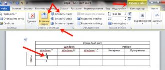
Alternatively, you can transfer the table from Excel to Word and do everything there. In Microsoft Word this is done much easier, using a numbered list. This approach is not quite the same, but it also allows us to solve the problem.

This is how you can number rows and columns in Excel. Each option for solving this problem is good and convenient in its own way, so choose which one you like best. Write in the comments whether this article helped you, and ask all your questions on the topic discussed.

Using the ROW function

These are already the first attempts at automatic line numbering in Excel. Simple formula and great results:

Select the first cell
Write the formula =ROW()-1 in it. Here we subtracted one from the function result - this is the number of lines that the header occupies. You subtract the number you need so that the first row of the array contains one
Copy the formula to the remaining cells of the column

Unlike previous methods, using the function allows you to sort the table and not redo the numbering later. All lines are renumbered automatically in the correct order.

How to automatically number rows using the Progression tool

You can automatically number table rows using the progression function without using a fill marker, i.e. There is no need to grab it and drag it. To do this, select the first cell of the list (after inserting one there), open the progression tool, switch it to the column position, indicate the final value (the number of all rows that need to be numbered). Finally, click OK and see that all rows of the table are numbered. It must be said that when deleting or vice versa, when inserting a new line, the numbering is broken. It is convenient to restore the numbering by again dragging the fill marker.

Numbering using progression

Number lines with COUNTA function

How to number rows in Excel in order when there are gaps in the table? Write down a formula similar to mine: =IF(B2<> "" ;COUNT($B$2:B2); "" ).

We get the following result:

More about the COUNTA function here.

Manually

It is important to know how to do numbering in order automatically in Excel, but performing such actions manually can reduce table processing time for small volumes.

Reverse numbering

Let's look at how to do numbering in Excel in reverse order. To do this you need:

Fill in the first 2 cells to determine the sequence of the spreadsheet.
Select range.
Point the mouse to the lower right corner, where the cursor changes to a black plus sign.
While holding down the left mouse button (LMB), drag the range down.

Note: The spreadsheet is able to fill a range even with negative numbers.

In order

To number rows in Excel using manual autofill, you must:

In the first two cells, enter 2 values.
Select the range and place the cursor in the lower right corner of the selected area.
While holding down the LMB, drag the range to the limit value.

With a gap

To autofill lines with numbers with a certain interval, the user needs:

Set the first and second values in the corresponding cells, and the step (spacing) can vary.
Select the range and move the mouse to the lower right corner to place a specially designated cursor.
Hold LMB and stretch the interval to the maximum mark.

Numbering Rows Using Subtotals

You can use the SUBTOTAL function instead of COUNT. The advantage is that when filtering, the function will correctly recalculate the line numbers so that the numbers in the displayed values are in order. Write down the formula according to my sample: =INTERMEDIATE TOTAL(3,$B$2:B2) and copy it to all cells. The range is numbered:

Now look what happens when I filter the Regions by the value “Sicily”:

The line numbers have been recalculated to match the data set that is visible on the screen!

Automatically

The automatic method of numbering lines is appropriate for processing a large amount of information. In this case, 2 options are available: using a function and a progression. Both methods make your work easier when considering the question of how to automatically number rows in Excel.

Using the function

To get the result, you need to know how to add numbering in Excel using a function. To use a mathematical tool, the user writes the formula: =ROW (argument).

In the first case, the user needs to click on the cell and enter the expression: =ROW (cell address), for example: =ROW (C3). The next step is to move your mouse to the bottom right corner of the range to get a black plus. While holding the LMB, you need to drag it down to create automatic numbering.

In the second case, leave the argument value empty, i.e. The function looks like this: =ROW(). The further algorithm is similar to the first step. Note: the difference between the first method and the second is that when you specify a specific address in brackets, the table automatically starts calculations from the line number specified in the address, regardless of the address of the selected cell. For example, cell H6 is selected, and the function contains the address H2. The application calculates from the number “2”. If there is no argument in the formula, the table calculates the range from the row specified in the address of the selected cell. For example, active cell: F4. Accordingly, Excel starts automated numbering with the number “4”.

In the third case, you should specify the function in the following format: =ROW()–2. Accordingly, to autofill lines starting with the number “1”, you need to specify the number of cells up to the first line.

Using progression

The built-in toolkit suggests using progression to automatically number rows in Excel. To do this, the user should:

Activate the cell and specify the first value.
Find the Fill tool on the Home tab and select Progression.
In the window that appears, prompting you to select the options: “By rows” or “By columns” - check the second item.
Specify the limit value and step (a number that affects the subsequent value in autofill).
Confirm the action with OK.

Note:

To create automatic numbering of odd numbers: specify step = 2, the first number in the series is odd. For example, initial value=1, step=2, limit value=7. Then the autocomplete looks like this: 1,3,5,7.
To create autocomplete for even numbers, the user proceeds in the same way, only the initial value is an even number.

"Progression"

You also need to figure out how to automatically number rows in an Excel table. Apply the Progression function. You will spend much less effort, since there will be no manipulations with the fill marker.

Your actions:

enter the initial parameter in the cell;
select this cell and the others that need to be numbered;
go to the “Home” - “Editing” tab, click “Fill”;

you need the “Progression” item, decide on its type;
set the location for the fill;
specify the filling step (by what amount the value will change) and the limit value for filling (how many cells should be numbered);
Click OK.

How to number a table in Excel by changing the value?

It's simple. Let's say you need a step with a gap of 3:

enter a numerical sequence into the first cells, each participant will be 3 more than the previous one. For example, 3, 6, 9, 12;
highlight the above-mentioned cells and those that should be numbered;
call the "Progression" command. Make a choice in favor of arithmetic and put the number 3 in the “Step” line;

confirm the action OK.

Reverse numbering

To create a reverse order, you can use the method described above:

Enter the first numbers of the sequence, for example, 10 9 8.

Select them and drag the marker down.

Numbers will appear on the screen in reverse. You can even use negative numbers.

Excel implies not only a manual method, but also an automatic one. Manually dragging the marker with the cursor is very difficult when working with large tables. Let's consider all the options in more detail.