Sorting in Excel is used to visualize data and organize it, which greatly facilitates the perception of information presented in tabular form. The need for this function arises when working with accounting statements, inventory lists and construction estimates.
Often the problem can be the issue of ordering numbers from high to low or vice versa. In fact, the criteria for organizing information in Excel are different: date, time, cell color or font type. Most often, when learning how to work with spreadsheets, examples are considered that present lists of employees or products, since in practice it is necessary to sort alphabetically very often. You can sort in the program according to two different parameters.
How to sort alphabetically
Since in most tables the numerical parameters are tied to some text - a surname or product name, it is convenient to arrange them alphabetically. Let's look at the features of working with this tool in the Excel editor using the table “Nutrient content in fruits and vegetables” as an example.
In order to sort the names of vegetables and fruits alphabetically, you need to select the first column by clicking on its heading. Next, you need to go to the “Editing” toolbar and open the “Home” tab, on which there is a special “Sort and Filter” button. To order the names in the first column from A to Z or vice versa, just select the appropriate sorting command in the drop-down menu. If data about other products is added to the Excel table, automatic sorting will work.
Custom data sorting
Simple sorting by one parameter is not always applicable or effective. It often happens that this parameter has the same values. For example, we sorted the items alphabetically, but we have several identical items on the list, but at different prices. In this case, after sorting, the data can be arranged in a random order.
Let's try adding a second sorting option. For example, so that if the name matches, the second stage of ordering is triggered.
- To implement our plan, go to the same “Sorting and Filter” tab, as with simple sorting. But then, for our current task, we will need to select the “Custom sorting...” item.
- A settings dialog will appear. Please note that if your table contains headers, this will need to be noted in the settings. To do this, check the box next to “The list contains headings.”
- In the “Column” column, you must indicate the name of the desired column by which the data is sorted. In the example given, this column is called “Name”.
- Then you need to select the “Sorting” option. It is responsible for the principle by which the data will be organized. There are four options in total: by cell color, by cell icon, by font color and by data value.
The most commonly used option is by data values. Therefore, this parameter is set by default. In our situation, we also need to sort by values, so we don't need to change anything.
- Then pay attention to the “Order” item. Since we have text information, we need to click on “From A to Z” (if necessary, you can select the other way around).
- Now we need to complicate the sorting by adding a second condition – by price. To do this, click on the “Add Level” button in the form of a plus in the lower left part of the window.
- Another line called “Then By” will be added. Here you need to do the same thing - fill out the columns in accordance with the conditions of the second stage of sorting.
In our example, the column name is “Price, rub.” We will sort by value, and the order will be “Ascending” (or vice versa, if required).
- In a similar way, you can set sorting by an unlimited number of conditions in the order of their priority. After all parameters have been set, confirm the action by clicking “OK”.
- As a result of these actions, the data is now sorted according to two criteria. First by name, and if the values coincide, by price.
Note: Sorting can be done not only by columns, but also by rows.
- In order to do this, go to the “Options” tab.
- A window with settings will appear in front of you. To change the sorting from columns to rows, select the appropriate option. Then confirm the changes by clicking “OK”.
- Next, we proceed according to the above scheme - indicate the required sorting parameters and click “OK”.
How to sort by ascending values in Excel
Simple ascending distribution in Excel is carried out in the same way as alphabetical distribution. After selecting the desired column at the top of the main window on the “Home” taskbar, in the “editing” section, select the “Sort and Filter” button, which has an additional menu. In the list that opens, you must select the appropriate option. When data in an Excel table needs to be sorted from largest to smallest, it should be sorted in descending order, otherwise select the “Sort in ascending order” option.
If the data range consists of two or more columns, when sorting, a dialog box should appear on the screen to choose what to do next. If the user needs to sort the data in the entire table in ascending order, then “automatically expand the selected range” should be specified; in the second case, the data will be ordered only in the selected column.
Sort by specified numeric values
Analysis of the work done, sales volumes, profit growth, student performance, purchases of additional materials is accompanied by the identification of parameters that have maximum and minimum indicators. Of course, if the table is small, then the user will be able to simply find the best indicator. But in cases where Excel has an excessively large number of rows and columns, without using built-in functions that allow you to sort the table, you can find the desired indicator, but you will have to spend a lot of work time.
You can do a much more practical thing, read the information on how to sort in Excel, and immediately begin to practically consolidate the knowledge gained.
Filter ascending and descending
It's very easy to sort data in ascending or descending order. You just need to find out whether the table is accompanied by numerous formulas. If this is the case, then it is best to move the table to a new sheet before sorting the data, which will avoid violations in formulas or accidental breaking of links.
In addition, a backup version of the table never hurts, since sometimes, if you get confused in your own reasoning and want to return to the original version, this will be difficult to do unless a preliminary copy is created.
So, first you need to select the table to be analyzed. Next, go to a new sheet, right-click, and then click on the “Paste Special” line. A window with parameters will appear on the screen in front of the user, among which you need to select the “Value” option, and then click “Ok”.
Now the duplicate version has been created, so you can proceed to further actions. To fully understand how to sort a table in Excel in ascending order, you need to select the entire table again, then go to the “Data” tab, where among several tools there will be the desired “Sort”, which you need to click on.
In the options window that opens, there is a line “My data contains headers.” Near it there is a small window in which you should check. All that remains is to set the column to be analyzed in the windows below, as well as the desired sorting option: ascending or descending. Next, we agree with the set parameters, after which the table will instantly demonstrate the desired result, eliminating many hours of grueling work.
If you need to sort not the entire table, but only one column, the steps will be almost the same, with the exception of only two points. Initially, you should not select the entire table, but only the desired column, and later, when Excel offers to automatically expand the range in order to sort, you need to refuse this by checking the box next to the phrase “Sort within the specified range.”
How to sort by date
In tables that display certain transactions in chronological order, they often need to be sorted by date. Because a date is a combination of integers represented in a specific way, proper sorting requires that the appropriate cell format be selected. If the format is incorrect, the program will not be able to recognize the date values, so it will not be possible to order them.
To sort table rows by date in the Excel editor, you need to perform the following sequence of actions:
- Select any cell in the column that contains the dates you want to sort.
- In the “Home” tab, find the “Sort and Filter” button, hover over it and select one of the proposed actions in the drop-down list. This can be a distribution from new to old, when the most recent dates and values attached to them are at the beginning of the list, or vice versa from old to new.
What can you sort?
The sorting function will be useful if you need to arrange cell values alphabetically or in ascending/descending order
Excel can sort data by text (alphabetical or vice versa), numbers (ascending or descending), date and time (new to old, and vice versa). You can sort by one column or several at the same time. For example, you could first sort all customers alphabetically, and then sort them by the total amount of their purchases. In addition, Excel can sort by custom lists or by format (cell color, text color, etc.). Usually sorting is applied only by columns, but it is possible to apply this function to rows as well.
All specified settings for this option are saved with the Excel workbook, allowing you to resort the information when you open the workbook (if necessary).
Sort by cell color and font
If a certain range of tabular data is formatted using different font colors or fills, the user can sort the rows by the color of some of the cells. You can also organize your data by a set of icons that were created using conditional formatting. In any case, it can be done like this:
- Use the mouse cursor to select one of the cells with data in the desired column.
- On the “Home” tab, in the “Editing” functional group, find the “Sorting and Filtering” button and select the “Custom Sorting” command in the additional menu.
- In the window that opens, first specify the column in which you want to sort the data, and then the sort type. This could be a cell color, a font color, or a conditional formatting icon.
- Depending on the selected type of sorting in the order group, you must select the desired icon or fill or font shade.
- The last parameter that needs to be specified is the location sequence (top or bottom).
Since there is no specific order of icons or colors in the editor, you need to create it yourself. To do this, you must click the “Add Level” button and then repeat these steps for each color or icon separately, excluding those that do not need to be included in the sorting,
How to set up a filter in a table
In addition to sorting, Excel has the ability to filter information. This function makes it possible to display only part of the selected data, while the rest of the information can be hidden. At the same time, hidden data is not lost anywhere, and it can be made visible again at any time when required.
Let's see how this works in practice.
- To do this, click on any cell (it is better if it is the table header). After that, go to the “Sorting and Filter” tab and select the “Editing” block here. In the list of functions that opens, you need to click on “Filter”.
- As a result, cells with column names should be marked with a special icon. This is a square, in the center of which there is a triangle with the point down.
- Now select the column you want to filter and click on the filter icon. For example, the task is to filter data by price.
- Let's say we only need product names at a price of 6,990 rubles. In this case, uncheck the boxes next to the remaining values.
- As a result, only information related to the selected price should remain in the table. You can tell that a filter is active in a column by the changed filter icon in the lower right part of the cell.
The task can be complicated by adding additional filtering conditions . Let's say you want to leave visible only items whose sales in the 1st quarter exceed a certain value, for example, 3 million rubles.
- To do this, you need to click on the filter icon in the “Total for 1 sq., rub.” cell. and select the desired values by checking the boxes. As a result, only the required information will remain in the visible part of the table.
- Also, when there is a lot of data, instead of selecting the required values, you can set a filtering condition. To do this, go to the filter window for the desired column, click on the “select” parameter, set the “greater than” condition and indicate the desired numeric value.
Sort by multiple columns in Excel
If there is a need to sort data in the Excel editor by two or more columns, you should, as in the previous case, select a data range and open the “Custom Sorting” window. Next, in the first group, you should note the heading of the column in which the data needs to be sorted first. The second group remains unchanged, and in the third you must specify the desired sorting type.
To specify sorting criteria for the second column, you need to add another level. As a result, the number of levels will correspond to the number of columns by which you need to sort the data.
By color
Formatting data by date or color is not much different from each other. You need to select the table, go to the “ Sorting ” menu and select “ Options ”. In the subsection, select the “ Sort by color ” option. After this, in the appropriate window you need to set the color shade from which the sorting will begin (i.e., it will be at the top or bottom of the table). After confirming the action, the editor will display an edited table in which the specified color will be located at the top or bottom.
In this way, particularly important or critical points can be marked with the appropriate color to highlight them later.
Dynamic table sorting in MS Excel
When performing some tasks in Excel, you need to set automatic sorting, which requires the presence of formulas. Depending on the type of data in the range used, dynamic sorting can be specified in three ways:
- If the information in the cells of a column is represented by numbers, the SMALL and ROW functions are used. The first finds the smallest element from the array, and the second determines the ordinal number of the row. In this way a sequence is formed. The formula is written as follows: =SMALL(A:A,ROW(A1)).
- When the cells contain text, the first formula will not work. To sort in this case, it is advisable to use the formula: =COUNTIF(A:A;”<“&A1)+ COUNTIF ($A$1:A1;”=”&A1).
- To automatically sort text information, text information also uses an array formula: =INDEX(List; SEARCH(SMALL(COUNTIF(List; “<“&List); ROW(1:1)); COUNTIF(List; “<“&List) ; 0)). Here List is the specified range.
Standard sorting
You can sort a table in Excel as standard; the procedure includes 3 options:
- alphabetically (from A to Z);
- increasing;
- descending
This is convenient when working with specific and large blocks of information. For example, sales volumes or calculation of income or expenses. Of course, in a 4x4 table the user will be able to quickly find the desired number, but with dimensions 44x44 it is more difficult to do this - in this case, sorting is used.
Changing numbers or other data in ascending or descending order is simple. First of all, you should determine the presence of formulas in the table . If they are, then it is best to transfer the data to a new sheet so as not to change the cell settings. After completing all preparatory operations, you need to select the desired table and go to the “ Data ” panel. Sorting item is located in this menu .
When you select this menu, a list will open with data parameters , select a specific column for analysis and the desired sorting option - ascending or descending . Next, we confirm the action, as a result of which the table will be displayed with the necessary parameters.
Advice! If there are formulas in the table, then you need to put a cross next to the line “ My data contains headers .”
You can arrange text alphabetically in the same way, you just need to select the appropriate filter option (in different versions of Excel it is labeled differently: A-Z or A-Z).
How and where to use the “Parameter Selection” function in Excel
How to remove sorting in Excel
To cancel single sorting of a data range, just click the “Cancel input” button in the left corner of the screen. It happens that changes to a file have been saved and it is impossible to undo the action. How can I remove sorting in this case?
If, after complex manipulations with the table, it needs to be returned to its original form, before sorting, you should specially create an additional column in which the row numbering will be reflected. After completing a complex analysis of the numeric and text data presented in the table, in order to undo all the operations performed, it will be enough to sort by the created column.
How to remove a filter in a table
- To return hidden data and remove column filtering options, click on the filter icon in the desired column and click “Clear filter”.
- If you are faced with the task of removing absolutely all filtering parameters in the table, go to the “Sorting and Filter” section and click the “Clear” button.
- To basically remove a filter from the table, in the same “Sorting and Filter” section, click on the “Filter” button, opposite which there is a checkmark indicating that this tool is now active in the table.