The guide describes various methods to quickly merge two or more cells in Excel without losing data.
In Excel spreadsheets, you may often need to combine two or more cells into one larger one. For example, this can be useful for better presentation of data. In other cases, there may be too much content to display in one table cell, and you decide to join it with adjacent empty ones.
Whatever the reason, merging cells in Excel is not as simple as it may seem. If at least two of them you are trying to merge contain data, then the standard merge function will only retain the top left value and destroy the data in the others.
- Merge and center function.
- Other methods.
- Limitations and features.
- How to merge cells in Excel without losing data
- How to merge columns without losing data?
- Convert multiple columns into one using Notepad.
- How to quickly find merged cells
- How to split cells in Excel
- Alternatives to merging cells.
But is there a way to merge cells in Excel without losing data? Of course have.
Merge and center function.
The fastest and easiest way to join two or more cells in Excel is to use the built-in Merge and Center option. The whole process takes just 2 quick steps:
- Select the range you want to merge.
- On the Home tab, click
In this example, we have a list of fruits in A2, and we want to combine it with a couple of empty cells on the right (B2 and C2) to create one large one that will fit the entire list.
After you click the button, A2,B2 and C2 will turn into one and the text will be centered, like in this screenshot:
Methods of combining
All methods for combining columns in Excel can be divided into two categories, which differ in the principle of execution. Some involve the use of formatting tools, while others use program functions.
If we talk about the ease of performing the task, then the first category is the undisputed leader. But, unfortunately, it is not always possible to achieve the desired result using formatting settings. That is why it is recommended to read the article to the end in order to determine for yourself the most suitable method for completing the task. Well, now let's move directly to how to combine data in columns in Excel.
Other methods.
To access several more integration options that Excel provides, click the small drop-down arrow next to the button and select the option you want from the drop-down menu:
Merge by rows —merge selected cells in each row separately:
Merge cells - merges the selected cells into one without centering the text. The default text will be left aligned and the number right aligned. Note. To change the text alignment after merging, simply select the desired alignment from the Home tab.
And another good way to merge cells is through the context menu. Select the appropriate area with the cursor, right-click, and then select “Format Cells” from the list.
In the window that appears, select “Alignment” and check the box next to “Merge Cells”. Here you can also set other parameters: text wrapping by words, auto-width selection, horizontal and vertical text orientation, various alignment options. After everything is set, click “OK”.
I think you remember that the formatting window can also be called up with the key combination CTRL + 1.
Cell Format
The Excel command Right Mouse Click → Format Cells → Alignment → Display → Merge Cells removes borders between cells in the selected range. The result is one large cell. The picture shows the union of cells of one row and three columns.
You can combine any rectangular range in the same way. After merging cells, the contents are often centered. On the ribbon in the Home there is even a special command Merge and place in center .
Beginner Excel users often use this command to center the table title.
It looks nice, but is extremely impractical. If you select a column using the Ctrl + Space , the range will expand to cover all the columns that the merged cell covers. Other problems will arise: when copying, it does not work in an Excel table, it is impossible to automatically adjust the column width, etc. In general, merging cells promises a lot of inconvenience in further work. Therefore, in most cases it is better not to merge cells.
Limitations and features.
There are a few things to keep in mind when using Excel's built-in cell merge functions:
- Make sure that all the data you want to see is entered in the leftmost cell of the selected range. After all, only the contents of the upper left cell will be saved, the data in all others will be deleted. If you want to integrate two or more cells together with data in them, check out the next section just below.
- If the button is inactive, the program is most likely in editing mode. Press Enter to finish editing, and then try merging.
- None of the standard join options work for data in an Excel table. First you need to convert the table to a regular range. To do this, right-click the table and select Table > Convert to Range from the context menu. But then follow the instructions.
Center alignment (without merging cells)
To position the text in the middle of the line, use the center alignment .
- Place the text in the left cell of the row where the alignment should occur.
- Select the required number of cells to the right.
- Call the command Right mouse button → Format cells → Align → horizontal → center selection .
Externally, the result is the same as when merging, only all the cells will remain in their place. There are a couple of nuances.
- It is not always clear which cell a record is in.
- Aligning to the center can only be done horizontally, not vertically.
In most cases, it is better to use center alignment merging cells .
The cell format only affects the display of data. In fact, you often have to combine content from different cells. Next, we’ll look at how to combine data from several cells into one in Excel.
How to merge cells in Excel without losing data
As mentioned, standard merge functions only save the contents of the top left position. And although Microsoft has made quite a few improvements in the latest versions of the program, the merge feature seems to have escaped their attention. And this critical limitation remains even in Excel 2020 and 2020. Well, where there is no obvious way, there is a workaround 
Method 1: Merge cells in one column (Align function)
This is a fast and easy connection method without losing information. However, this requires that all the data being joined be in the same area in the same column.
- Select all the table cells you want to merge.
- Make the column wide enough to contain all the content.
- On the Home tab, use Fill > Align >. This will move all content to the very top of the range.
- Choose an alignment style depending on whether you want the resulting text to be centered or not.
If the resulting values are spread across two or more rows, make the column a little wider.
This merging method is easy to use, but it has a number of limitations:
- You can only merge in one column.
- It only works for text, numeric values or formulas cannot be processed this way.
- This does not work if there are empty cells between the merged cells.
Method 2: Use the CONCATENATE function
Users who are more comfortable using Excel formulas may like this method of merging cells. You can use the CONCATENATE function or the & operator to first concatenate the values and then optionally concatenate the cells themselves.
Let's say you want to connect A2 and B2. There is data both there and there. To avoid losing information during a merge, you can use any of the following expressions:
=CONCATENATE(A2;" ";B2)
=A2&" "&B2
We will write the formula in D2. And now we already have as many as 3 positions: two original and one combined. Next, a few additional steps are required:
- Copy D2 to the clipboard (you can use CTRL + C).
- Paste the copied value into the top left position of the range you want to merge (into A2). To do this, right-click it and select Paste Special > Values from the context menu.
- Now we can delete the contents of B2 and D2 - we won’t need it anymore, it will only get in the way.
- Select the positions you want to connect (A2 and B2), and then - .
You can connect multiple cells in the same way. Only the CONCATENATE formula in this case will be a little longer. The advantage of this approach is that you can use different delimiters in the same expression, for example:
=CONCATENATE(A2; ": "; B2; ", "; C2)
You can find more examples in this tutorial - CONCATENATE in Excel: How to combine text strings, cells and columns.
Excel JOIN (TEXTJOIN) function
JOIN function also appeared in Excel 2016 and immediately solved all the problems of gluing cells together: specifying an entire range, inserting a separator, and even skipping empty cells in the range so as not to duplicate the separator.
Function syntax.
COMBINE(delimiter, skip empty, text1,…)
separator – a separator that is inserted between cells
skip_empty – if 0, then empty cells are included, if 1, they are ignored. Usually set to 1 so as not to duplicate the separator.
text1;... – link to a range or individual cells for concatenation.
Excel's MERGE function is the best solution for merging cells.
How to merge columns without losing data?
Let's say you have information about clients where the first column contains the last name and the second column contains the first name. You want to combine them so that the last name and first name are written together.
We use the same formula approach that we just looked at above.
- Insert a new column into your table. Place your mouse pointer on the column header (D in our case), then right-click and select " Insert " from the context menu. Let's just call him "Full Name".
- In D2 write the following: =CONCATENATE(B2," ";C2)
B2 and C2 are the last name and first name, respectively. Please note that there is also a space added between the quotes. This is the separator that will be inserted between the concatenated names. You can use any other character as a delimiter, such as a comma.
Likewise, you can merge data from multiple cells into one using any separator of your choice. For example, you can combine addresses from three columns (street, city, zip code) into one.
- Copy the formula to all other positions in the Full Name column.
- We combined first and last names, but it's still a formula. If we delete the First Name and/or Last Name, the corresponding linked data will also disappear.
- Therefore, we need to convert it into a value so that we can remove unnecessary things from our sheet. Select all the filled cells in our new column (select the first one and apply the key combination Ctrl + Shift + ↓).
- Copy the selection to the clipboard (Ctrl + C or Ctrl + Ins, whichever you prefer), then right-click anywhere on the same selection (Full Name) and select Paste Special from the contextual menu. Select the Values radio button and click OK.
- Remove the First Name and Last Name columns, which are no longer needed. Click heading B, press and hold Ctrl and click heading C (an alternative is to select any cell on B, press Ctrl + Spacebar to select the whole thing, then Ctrl + Shift + → to select C).
After that, right-click any of the marked columns and select “Delete” from the context menu.
Great, we've combined the names from two columns into one ! Although it took quite a lot of effort and time
Conclusion
The process of combining columns in Excel can be done in different ways.
The simplest are the first and second methods. However, the most functional way that allows you to save data is the third.
If you have Telegram, you can now download any software or game through our bot, just follow the link and try it!
« Previous entry
Convert multiple columns into one using Notepad.
This method is faster than the previous one, it does not require formulas, but is only suitable for combining adjacent columns and using the same separator for all data.
Here's an example: we want to merge together 2 columns with first and last names.
- Select the source data: press B1, then Shift + → to select C1, then Ctrl + Shift + ↓ to select all first and last names.
- Copy the data to the clipboard (Ctrl + C or Ctrl + Ins).
- Open Notepad: Start -> All Programs -> Accessories -> Notepad.
- Paste data from the clipboard into Notepad (Ctrl + V or Shift + Ins)
5. Copy the tab character to the clipboard. To do this, press Tab to the right in Notepad. The cursor will move to the right. Select this tab with your mouse. Then transfer it to the clipboard using Ctrl + X.
6. Replace the tab characters in Notepad with the desired delimiter.
You need the Ctrl+H combination to open the Replace dialog box, paste the tab character from the clipboard into the What field. Enter a separator, such as space, comma, etc. in the "What" field. Then click the “Replace All” button. Let's close.
- Press Ctr + A to select all text in Notepad, then Ctrl + C to copy to the clipboard.
- Go back to your Excel sheet (you can use Alt + Tab), select only B1 and paste the text from the clipboard into your table.
- Rename Column B to "Full Name" and remove "Last Name".
There are more steps than the previous option, but try it yourself - this method is faster.
Combining text with line breaks.
Most often, you would separate connected text elements with punctuation and spaces, as shown in the previous example. However, in some cases you may need to separate them using a line feed or carriage return. A typical example is combining postal addresses from information in separate columns.
The problem is that you can't simply enter a line break like a regular character, and so a special CHAR function is needed to supply the appropriate ASCII code to the concatenation formula:
- On Windows, use CHAR(10), where 10 is the ASCII code for newline.
- On a Mac system, use CHAR(13), where 13 is the ASCII code for carriage return.
In this example, we have address parts in columns A through F, and we concatenate them in column G using the concatenation operator "&". Concatenated elements are separated by a comma (","), a space (" ") and a newline CHAR(10):
=A2&" "&B2&CHAR(10)&C2&CHAR(10)&D2&", "&E2&" "&F2
Note. When using line breaks to separate concatenated values, you must enable the Text Wrap for the result to display correctly. To do this, press Ctrl + 1 to open the Format dialog box, go to the Alignment tab, and check the Wrap Text checkbox.
In the same way, you can separate related parts with other symbols, such as:
- Double quotes (") - CHAR(34)
- Slash (/) - CHARACTER(47)
- Asterisk (*) - SYMBOL(42)
Although it is easier to include printable characters in the concatenation formula by simply typing them in double quotes, as we did in the previous example.
In any case, all four of the expressions below give the same results:
=A1 & CHAR(47) & B1
=A1 & "/" & B1
=CONCATENATE(A1, CHAR(47), B1)
=CONCATENATE(A1, “/”, B1)
How to quickly find merged cells
To find such areas, follow these steps:
- Press Ctrl+F to open the Find and Replace , or search the ribbon for Find and Select > Find.
- On the Find tab, click Options > Format.
- On the Alignment tab, select the Merge Cells and click OK.
- Finally, click Find Next to move to the next merged cell, or Find All to find them all on the worksheet. If you choose the latter, Microsoft Excel will display a list of all the joins found and allow you to move between them by selecting one of them in this list:
What problems arise when using merged cells
As has already been said, you should be careful when using merged cells, as they limit the functionality of Excel and can cause trouble in the future. If you do decide to use merged cells, always remember the following points:
- If a range contains merged cells, you will not be able to use sorting or filtering in that range.
- It will also be impossible to convert such a range into a table (format as a table).
- You can also forget about automatically adjusting the cell width or height. For example, if there is a merged cell A1:B1, then it will no longer be possible to align the width of column A.
- If you use hotkeys for navigation, for example, go to the beginning and end of the table using the Ctrl + up and down arrow key combination, then the transition will fail and the cursor will “rest” on the merged cells.
- If you select columns (or rows) using the hotkeys Ctrl (Shift) + Space , then if you have merged cells, you will not be able to select 1 column (or row).
How to merge without losing data
The previously described options for merging table elements involve deleting all the data in the cells, with the exception of one. The only thing that remains after this procedure is the value located in the upper left cell. However, in some cases it is necessary that after processing all the information from the cells involved in the merging process is preserved. Excel developers have foreseen this and provided the user with a special concatenation function, with which cells can be combined without losing data.
The main purpose of the function is to combine a range of rows containing data into a single element. Here's what the formula for the tool that allows you to do this looks like: = CONCATENATE(text_1;text_2;…)
The function argument can be either a specific value or the coordinates of a cell in a table. We will use the last option, since it will help us solve the problem correctly. The maximum number of function arguments is 255, which is more than enough.
For example, let's take the same table with the names of goods. Now you need to combine all the data located in the first column in such a way that nothing is lost.
- Place the cursor in the cell in which the result will be displayed after the procedure. Then click on the button that is responsible for inserting the function.
- After the Function Wizard appears on the screen, select the line “CONNECT” from the list, and then click OK.
- Now you need to fill in the function arguments. As is already known, their maximum number is 255, however, in our case, only 5 will be enough (the number of rows that are planned to be combined). In the window that appears for managing function arguments, click on the first field, then on the first cell of the row that is included in the range we have selected. If everything is done correctly, the coordinates of the selected cell will appear in the first field, and its value will appear next to it. Next, you need to repeat the procedure with all other cells participating in the merger. After that, click the “OK” button.
- After damage, all values of the selected cells will be inserted into the specified cell in one line, without hyphens or spaces. This, of course, looks ugly, so everything needs to be corrected. To do this, you need to select the cell in which the formula is located and click on the “Insert Function” button again.
- The argument settings window will appear on the screen again. In each of the fields, after the cell address you need to add special characters &” “ . But, in the last field only the address should be indicated. These characters act as a kind of space character when using the concatenation function. It is for this reason that they are not needed in the last field. After everything is done, confirm the action by pressing the OK button.
- Now there are spaces between the values, just like we wanted.
There is another method of combining elements while preserving their values . In order to implement it in practice, there is no need to use the concatenation function; it will be enough to use the usual formula.
- First, you need to write an equal sign (“=”) in the cell in which we plan to display the final result. Next, click on the first cell located in the column from the selected range. Its address should be displayed in the formula bar, as well as in the cell in which we write the formula. Now we write special characters &” “&.
- After that, add the remaining cells from the rows of the column selected for merging to the formula in the same way. The result should be the following formula: A2&” “&A3&” “&A4&” “&A5&” “&A6& .
- In order to display the result, all you have to do is press the Enter key. After this, you can see that using this formula, we achieved exactly the same result as in the case of using the clutch function.