Spreadsheet programs like Excel rarely care about the appearance of the data until it's all entered into a worksheet and saved. Only after this does the desire arise to make the information understandable and easy to view. In this article you will learn how to create a table in Excel?
Once you've decided what type of formatting to apply to portions of your worksheet, you need to select the cells and select the appropriate tool or menu item. But first of all, you should learn how to select cells or create cell selections.
Keep in mind that entering data into cells and formatting them are two completely different tasks in Excel. You can change data in formatted cells while still applying existing formatting to new cells. You can format blank cells knowing that you will enter data into them in the future. This assumes that formatting will be applied to the data immediately as you type it.
How to create a table in Excel: Simple techniques for formatting cells
In this section, we'll look at table formatting tools that don't require you to first select cells. Click the Format as Table located in the Styles the Home tab . A collection of styles will appear on the screen, divided into three groups: Light , Medium and Dark . Each of these groups contains formatting colors of the corresponding intensity.
After clicking on one of the format thumbnails, the program will automatically try to highlight with a dotted line the range of cells to which the formatting will be applied. A table formatting dialog box will also appear on the screen.
The Format Table dialog box contains the Specify table data location , which specifies the range of cells selected by the program, and the Table with headers check .
If the program incorrectly selected the range of table cells to be formatted, then drag the mouse pointer over the required range, after which the address of the desired range will be displayed in the Specify the location of the table data . If your data table doesn't need headers, or if it already has headers but you don't want to add filtering drop-down lists to them, uncheck the Table with headers before clicking OK .
When you click OK in the Format Table dialog box, the selected format is applied to the range of cells. Table Tools contextual tabs appears on the ribbon , which includes a Design . A Quick Analysis Toolbox icon will appear near the lower right corner of the table.
Design tab, you can see how the table will look when using different formats (using Live Preview). Hover your mouse over one of the format icons in the Table Styles , and the table will change to match the selected style. To access all table formats, use the vertical scroll bar. Click the More Options —represented by a horizontal bar above a downward-facing triangle—to open the Tabular Format Gallery window. Hover your mouse over the style thumbnail under Light , Medium , or Dark to see how the table's appearance changes.
Whenever you select a format in the Table Styles gallery for one of the workbook's data tables, Excel automatically gives that table a generic name (Table 1, Table 2, and so on). To rename the data table to a more descriptive name, use the Table Name located in the Properties the Design tab .
Creating a table
- Select any cell containing data that will be included in the table.
- In the menu ribbon, select the Insert tab ; Tables group of commands that opens, select the Table .
- A dialog box appears in which Excel automatically suggests data range boundaries for the table
If this range needs to be changed, just select the desired data range with the cursor.
- OK.
Naming the table
By default, when you create an Excel table, it is assigned a standard name: Table1, Table2, etc. If there is only one table, then you can limit yourself to this name. But it is more convenient to give the table a meaningful name.
- Select a table cell.
- On the Design , in the Properties , enter a new table name in the Table Name and press Enter .
The requirements for table names are similar to those for named ranges.
How to create a table in Excel: Setting up table formats
In addition to allowing you to select a new table format from the Table Styles gallery, the Design tab includes a Table Style Options . This group contains checkboxes that allow you to further customize the appearance of the selected table format.
- Title line . Used to insert filter buttons into the column headers of the first row of the table.
- Total line . Insert a total row at the end of the table. This row displays the total values of all rows that contain values. To change the total function for a selected column, click on the corresponding cell in the last row to bring up a list of standard functions (sum, average, minimum or maximum, cardinality, standard deviation, and variance) and select the desired function.
- Alternating lines . Highlighting even table rows with shadows.
- First column . Make table row headings in the first column in bold.
- Last column . Makes the table row headings in the last column in bold.
- Alternating Columns . Highlighting even table columns with shadows.
- Filter button. Enables or disables the filter in the table header row.
When you've finished selecting and customizing the formatting of a table, click on a cell that doesn't belong to it, and the Table Tools , along with the Design , will disappear from the ribbon. If you decide to experiment with table formatting later, click on any of its cells, and the Table Tools along with the Design , will reappear on the ribbon.
Calculations in tables
You can add an additional summary row to the table, which will contain the results of various functions applied to the data of some or all fields. The procedure is as follows:
- On the Design , in the Table Style Options , select Total Row .
- In the new line that appears, Total [Total], select the field in which you want to process the data, and select the desired function from the drop-down menu.
To enter new records at the end of the table, select the totals row and use the right mouse button. A context menu will appear, in it you need to select Insert . If you enter data into the new line that appears, it will automatically participate in the recalculation of the totals.
In order to reduce the time it takes to add rows to the table, you can disable the totals row and add new data from a new row. In this case, the table will automatically expand its range.
To carry out calculations and place the results in a new field, just enter the formula in one cell of this field. Excel will automatically multiply it across all cells of this field. If Excel settings are set correctly, when you enter a formula, not cell addresses are written into it, but field names.
If instead of the field name on the screen, cell addresses are indicated in the formulas, you need to change the setting:
- Select the File tab or the Office button , depending on the version of Excel; then the Options .
- In the Formulas , in the Working with Formulas , check the Use table names in formulas .
- OK.
How to create a table in Excel: Formatting cells using the Home tab commands
Some worksheets require more precise formatting than is possible by clicking the Format as Table . For example, you might want a data table that has column headings in bold and a total row that is underlined.
The formatting buttons contained in the Font , Alignment , and Number the Home tab allow you to choose almost any formatting for your data table. Descriptions of these buttons are given in table. 1.
Table 1. Formatting buttons for the Font, Alignment, and Number groups on the Home tab
| Group | Button | Purpose |
| Font | Font | Displays a drop-down menu from which you can select any font for the selected cells |
| Font size | Opens a list from which you can select the font size for the selected cells. If the required size is not in the list, you can enter it from the keyboard | |
| Increase font size | Increases the font size for selected cells by one point | |
| Decrease font size | Decreases the font size for selected cells by one point | |
| Bold | Applies a bold style to selected cells | |
| Italics | Applies italics to selected cells | |
| Stressed | Applies an underline to selected cells | |
| Borders | Opens the Borders menu, where you can select borders for selected cells | |
| Fill color | Opens a color picker from which you can select a background color for selected cells | |
| Text color | Opens a color picker from which you can select a text color for the selected cells | |
| Alignment | Align text left | Aligns the contents of selected cells to their left border |
| Align Center | Centers the contents of selected cells | |
| Align text right | Aligns the contents of selected cells to their right border | |
| Decrease indent | Decreases the indentation of the contents of selected cells from the left border by one tab. | |
| Increase indent | Increases the indentation of the contents of selected cells from the left border | |
| Along the top edge | Aligns the contents of selected cells to their top border | |
| Align in the middle | Centers the contents of selected cells between the top and bottom borders | |
| Along the bottom edge | Bottom aligns cell contents | |
| Orientation | Opens a menu from which you can select the text angle and direction of the selected cells | |
| Wrap text | Wraps text that extends beyond the right border to the next line while maintaining the width of the cells | |
| Combine and place in the center | Merges the selection into a single cell and centers the content between the new right and left borders. Clicking this button opens a menu containing various merge options | |
| Number | Number format | Displays the number format applied to the active number cell. Click on the dropdown and you will see the active cell with the basic number formats applied to it |
| Financial number format | Formatting selected cells by adding a currency symbol, thousands separators, displaying two decimal places, and possibly enclosing negative numbers in parentheses. After clicking the button, a list of possible formatting options opens | |
| Percentage format | The numbers in the selected cells are multiplied by 100 and a percent sign is added to them. Decimal places are removed | |
| Delimited format | Spaces are used to separate thousands, two decimal places are displayed, and negative numbers are possibly enclosed in parentheses | |
| Increase bit depth | Adds a decimal to numbers in selected cells | |
| Decrease bit depth | Reduces the number of decimal places in numbers contained in selected cells |
Be aware of the tooltips that appear after you select one of the formatting command buttons with your mouse pointer. These tooltips not only provide a brief description of the button, but also display keyboard shortcuts that let you quickly add or remove attributes from entries in selected cells.
Using Excel cell borders and shading
Using Borders
Applying color and patterns
Using Fill
Using Borders
Cell borders and shading can be a good way to decorate different areas of a worksheet or draw attention to important cells.
To select a line type, click on any of thirteen boundary line types, including four solid lines of varying thicknesses, a double line, and eight types of dotted lines.
By default, the border line color is black when the Color box is set to Auto on the View tab of the Options dialog box. To select a color other than black, click the arrow to the right of the Color box. The current 56-color palette will open, in which you can use one of the existing colors or define a new one. Note that you must use the Color list on the Border tab to select a border color. If you try to do this using the formatting toolbar, you will change the text color in the cell, not the border color.
After selecting the line type and color, you need to specify the position of the border. Clicking the Outer button in the All area places a border around the perimeter of the current selection, whether it's a single cell or a block of cells. To remove all boundaries present in the selection, click the No button. The viewing area allows you to control the placement of borders. When you first open the dialog box for a single selected cell, this area contains only small markers indicating the corners of the cell. To place a border, click on the viewport where you want the border to be, or click the corresponding button next to that area. If you have multiple cells selected in a worksheet, the Inner button becomes available on the Border tab, allowing you to add borders between the selected cells. Additionally, additional markers appear in the viewing area on the sides of the selection, indicating where the inner borders will go.
To remove a placed border, simply click on it in the viewing area. If you need to change the border format, select a different linetype or color and click that border in the viewing area. If you want to start placing boundaries again, click the No button in the All area.
You can apply multiple types of borders to selected cells at the same time.
You can apply border combinations using the Borders button on the Formatting toolbar. When you click the small arrow next to this button, Excel will display a border palette from which you can choose the type of border.
The palette consists of 12 border options, including combinations of different types, such as a single top border and a double bottom border. The first option in the palette removes all border formats in the selected cell or range. Other options show a miniature view of the location of a border or combination of borders.
As a practice, try the small example below. To break a line, press the Enter key while holding down Alt.
Applying color and patterns
The View tab of the Format Cells dialog box is used to apply colors and patterns to selected cells. This tab contains the current palette and a drop-down pattern palette.
The Color palette on the View tab allows you to set a background for selected cells. If you select a color in the Color panel without selecting a pattern, the specified background color appears in the selected cells. If you select a color in the Color panel and then a pattern in the Pattern drop-down panel, the pattern overlays the background color. The colors in the Pattern drop-down palette control the color of the pattern itself.
Using Fill
The various cell shading options provided by the View tab can be used to visually design your worksheet. For example, shading can be used to highlight summary data or to draw attention to worksheet cells where data is entered. To make it easier to view numerical data by row, you can use the so-called “strip fill”, when rows of different colors alternate.
The cell background should be a color that makes the text and numeric values displayed in the default black font easy to read.
Excel allows you to add a background image to your worksheet. To do this, select the “Sheet” - “Background” command from the “Format” menu. A dialog box will appear allowing you to open a graphic file stored on disk. This graphic is then used as the background of the current worksheet, much like watermarks on a piece of paper. The graphic image is repeated, if necessary, until the entire worksheet is filled out. You can disable the display of grid lines in a worksheet by selecting the "Options" command from the "Tools" menu and on the "View" tab and unchecking the "Grid" checkbox. Cells that are assigned a color or pattern display only the color or pattern, not the background graphic.
Top of page
Top of page
Format a selection using the Mini Toolbar
To format a selected range of cells in Excel, you can use the Mini Toolbar.
To display the Mini Pane, select the cells that need formatting and right-click anywhere in the selection. The mini-panel will appear directly next to the context menu that opens. If you select a tool in the minibar, such as the Font or Font Size , the context menu will disappear.
The mini-panel contains most of the buttons from the Font the Home tab , with the exception of the Underline . In addition, there are buttons for right and left alignment and center alignment from the Alignment , as well as buttons for financial numeric and percentage formats, delimited format, decreasing and increasing bit depth from the Number . To apply one of these formatting tools to selected cells, click on the appropriate button.
Automatic creation
The application contains ready-made tables. They are already created with formatting. To use automatic creation, you need:
- Go to the “ Insert ” tab.
- Select an area for the table.
- Click on the appropriate command.
This tool can also be used through the “ Home ” panel. Then, you should select “ Format as table ”.
Rounding numbers in Microsoft Excel
In the open window there will be a list of styles, from which you need to click on the one you need. In order for formatting to be applied not to one cell, but to the entire selection, you must first select the range by holding down the left mouse button.
How to create a table in Excel: Cutting, copying and pasting cells
Instead of dragging and dropping and autofill, you can use the good old cut, copy, and paste to move and copy information on your worksheet. These commands use the Office clipboard as temporary storage where information remains until you decide to paste it somewhere. Thanks to the buffer, these commands can be used to move information not only to any worksheets open in Excel, but also to other programs running in Windows (for example, Word documents).
Using formulas in tables
It is thanks to the ability to use auto-calculation functions (multiplication, addition, etc.) that Microsoft Excel has become a powerful tool.
The best way to view complete information about formulas in Excel is on the official help page.
In addition, it is recommended that you read the description of all functions.
Let's consider the simplest operation - cell multiplication.
- First, let's prepare the field for experiments.
- Make active the first cell in which you want to display the result.
- Enter the following command there.
=C3*D3
- Now press the Enter key. After that, move the cursor over the lower right corner of that cell until its appearance changes. Then hold down the left mouse click with your finger and drag down to the last line.
- As a result of autosubstitution, the formula will fall into all cells.
The values in the “Total Cost” column will depend on the “Quantity” and “Cost 1 kg” fields. This is the beauty of dynamics.
In addition, you can use ready-made functions for calculations. Let's try to calculate the sum of the last column.
- First, select the values. Then click on the “AutoSums” button, which is located on the “Home” tab.
- As a result, the total sum of all numbers will appear below.
Moving using Cut and Paste commands
To move a selected range of cells using the Cut and Paste , follow these steps:
- Select the range of cells you want to move.
- Click on the Cut button, which is located in the Clipboard group of the Home tab (it shows scissors).
If you want, use the keyboard shortcut to cut.
When you select the cut command in Excel, the selected range of cells is surrounded by a blinking dotted line, and the following message appears in the status bar: Select a cell and press ENTER or select Paste.
- Move the cursor to the cell that should contain the upper left corner of the range where the information is moving (or click on it).
- Press the <Enter> to complete the operation.
You can also click the Insert Home Tabs or press the keyboard shortcut.
Please note that when marking the insertion location, you do not need to select a range that exactly matches the cut one. It is enough for the program to know the location of the upper left cell of the destination range - it will itself determine where to place the remaining cells.
Apply and remove cell borders on a worksheet
Using standard border styles, you can quickly add a border around cells or ranges of cells. If the predefined cell borders don't suit your needs, you can create a custom border.
Note:
The cell borders you want to apply appear on the printed pages. If you don't use cell borders, but you want the sheet grid line borders to be visible on printed pages, you can show the grid lines. For more information, see Printing with and without lines.
On the worksheet, select the cell or range of cells to which you want to add a border, change the border style, or remove the border.
On the Home
In the
Font
, do one of the following:
To apply a new or different border style, click the arrow next to the border
and select the border style you want.
Advice:
To apply a custom border style or a diagonal border, click the
More Borders
.
In the Format Cells
, on the
Border
, in the
Lines
and
Color
, click the line style and color you want.
In the Presets and Borders
, click one or more buttons to indicate the location of the border.
Two diagonal buttons available in the border
.
To remove cell borders, click the arrow next to the border
and select
No Border
.
Button » borders
" displays the last border style used.
You can click the border
(not the arrow) to apply the style.
If you apply a border to a selected cell, it will also be applied to adjacent cells that have a cell border border. For example, if you apply a border to the range B1:C5, cells D1:D5 receive a left border.
If you apply different types of borders to a common cell border, the Last Border Applied appears.
The selected range of cells is formatted as one block of cells. If you apply a right border to the range of cells B1:C5, the border appears only on the right border of cells C1:C5.
If you want to print the same border for cells separated by a page break, but the border only appears on one page, you can apply an inner border. So you can print a border at the bottom of the last line on one page and use the same border at the top of the first line on the next page. Follow the steps below.
Highlight the lines on both sides of the page break.
Click the arrow next to the border
and select
Other borders
.
In the presets section, click the Internal
.
In the border
in the diagram preview Remove the vertical border by clicking it.
Select the cell or range of cells on the worksheet for which you want to remove the border.
To deselect cells, click any cell on the worksheet.
On the Home
In the
Font
, click the arrow next to the
border
and select
No border
.
On the home
>
Border
>
Erase Border
, and then select the cells with a border that you want to erase.
You can create a cell style that contains a custom border, and apply that cell style if you want to display a custom border around selected cells.
On the Home
In the
Styles
, click
the Cell Styles
.
Advice:
If the
Cell Styles
doesn't appear, click the
Styles
, and then click the
More
next to the Cell Styles box.
Select New Cell Style
.
In the style name
Enter a suitable name for the new cell style.
Click Format
.
On the Border
In the
Line
in the
Style
, select the line style that will be used for the border.
In the Color
select the color you want to use.
In the border
Click the border buttons to create the border you want.
Click OK
.
Dialog style
In
the Style includes (by example)
, clear the check boxes for those formatting elements that you do not want to include in the cell style.
Click OK
.
To apply a cell style, follow these steps:
Highlight the cells you want to format using a custom cell border.
On the Home
In the
Styles
, click
the Cell Styles
.
Click the custom cell style you just created. the FancyBorderStyle button
in this picture.
To customize the line style or color of cell borders, or to erase existing borders, you can use the Draw Borders
". To draw cell borders, first select a border type, then a border color and line style, and then select the cells you want to add a border around. Here's how to do it:
On the Home
Next to Borders,
click
the arrow
.
To create outer boundaries, select Draw Borders
, for internal markings - item
Draw border lines
.
Click the arrow next to Borders
, select
Line color
and specify the desired color.
How to create a table in Excel: Copy and Paste
The method of copying a selected range of cells using the Copy and Paste is completely the same as described above. However, after selecting a range of cells, you have more options for placing it on the clipboard: click on the Home tab Copy , select Copy from the cell context menu that opens by right-clicking, or press the key combination.
The advantage of copying information to the clipboard is that you can paste it from the clipboard many times. Just note that instead of pressing the key as you did when you first pasted a copy, you should click the Home tabs Paste or press the key combination.
When you use the Paste , the program does not remove the dashed outline around the original range of cells. This is a signal that you can select additional insertion ranges (in the same or in a different document).
After selecting the first cell of the next range to copy to, click the Paste (this can be repeated as many times as you like). When you paste the last copy, press the key instead of selecting Paste or pressing the key combination. If you forget to do this, use the key to remove the dashed outline around the original range of cells.
Converting a table to a regular range
When working with tables, along with the advantages, there are a number of restrictions: you cannot merge cells, you cannot add subtotals, etc. If the table's calculations are complete and all you need is the data from it and perhaps some styling, the table can be quickly converted to a regular data range. To do this you need to follow these steps:
- On the Design , select the Tools .
- Select the Convert to Range .
- Click on the Yes .
How to create a table in Excel: Insertion options
If you click on the Paste Home tab or press a key combination to paste copied (not cut) cells into the clipboard, then at the end of the pasted range the program displays a paste options button with its own context menu. Clicking this button or pressing a key will open a palette with three groups of buttons: Paste, Paste Values, and More Paste Options.
Paste options let you control the content type and formatting in the pasted range of cells. The paste options (along with the corresponding keyboard shortcuts) are listed below.
Insert. All necessary information (formulas, formatting, etc.) is inserted into the selected range of cells.
Formulas . All necessary text, numbers, and formulas are inserted into the currently selected range of cells without formatting.
Formulas and number formats. The number formats assigned to the copied values are pasted along with the corresponding formulas.
Keep original formatting. The formats of the source cells are copied and pasted into the target cells (along with the copied information).
No frames. The content is pasted into the selected range of cells, but the borders are not copied.
Maintain original column widths. The width of the columns in the target range is adjusted to be equal to the width of the columns in the source range.
Transpose . Changes the direction of the inserted range. For example, if the contents of the original cells are located along the rows in one column of the worksheet, then the copied data will be located along the columns in one row.
Meanings. Only the calculated results of any formulas specified in the original range of cells are pasted.
Number values and formats. The calculated results of any formulas, along with the formatting specified for the labels, values, and formulas in the source range of cells, are pasted into the target range. This means that all labels and values in the target range will have the same formatting as those in the source range of cells, even if you lose all of the original formulas and retain only the calculated values.
Values and source formatting. The calculated results of any formulas are pasted along with the formatting of the original range of cells.
Formatting. Only the formats (without content) copied in the source range of cells are pasted into the target range.
Insert link. Formulas are created to reference source cells in the target range. This way, all changes made to the source are immediately reflected in the corresponding target cells.
Drawing. Only images within the copied range are pasted.
Related drawing . A link to images located in the copied range is inserted.
How to make data invisible in Excel
11/08/2012 Grigory Tsapko Useful tips
In some cases, it is necessary to make data in some cells invisible without deleting them. For example, intermediate results of calculations, zero values, the value of the parameter TRUE or FALSE, etc.
To do this, you can use at least two methods:
Firstly, the simplest thing is to set the font format in the cell to the same as the background color, that is, in the most common case, paint it white.
Secondly, you can change the data type, making it invisible. To do this, select the range of data cells required to hide, right-click and in the context menu that appears, select Cell Format Number tab → in the Number formats field: select (all formats) . On the right in the Type field: set three semicolons “;;;” (without quotes) and click OK .
The example below shows two data types: "Main" - visible, and ";;;" - invisible, as well as the sum of numbers, the same in both ranges.
Click on the picture to enlarge
To make data in cells visible, you need to do a similar operation. Select the required cells again and set the Type: Basic, or simply remove the “;;;” from this field.
These methods are applicable mainly to those cells in which the data must be hidden permanently. However, this does not always happen.
Let's look at a very common case where we need to make zero values in cells invisible. Moreover, we initially do not know where such values will appear.
We are talking about hiding zero values in various calculation models, planned budgets, etc. to improve the perception of information.
For example, we have a table in which the values are obtained by calculation. Let this be a planned sales budget, where revenue values for products are calculated as the product of the quantity of a particular product and its price.
If our goods are sold unevenly, then we will receive a final table of revenue with many zero values for those periods when there is no sale of goods.
The abundance of zero values interferes with the visual perception of information, periods when there is revenue merge with the general background, and visual analysis of the budget deteriorates.
In this case, to improve perception, it is necessary to hide zero values and leave only those revenue values when there is a sale of goods. Naturally, this process should occur automatically so that we do not have to manually change the font color or data type.
Click on the picture to enlarge
As you can see, the second option is much easier to accept.
To hide zero values, we can also use at least two methods.
First, we can use a formula based on the IF function.
So, for example, if we initially have the revenue value in cell B40 as the product of the quantity of goods sold from cell B5 by the price of the goods from cell B25 (B40=B5*B25), then the formula for hiding the zero revenue value in cell B40 will be look like this:
How to create a table in Excel: Deleting cell contents
A description of editing techniques in Excel would be incomplete without considering how to delete cells. There are two types of deletions you can perform on a worksheet.
Clearing cell contents. This deletes only the contents, but the cell itself remains in place. This way, the overall structure of the worksheet is not disrupted.
Deleting the cells themselves. The cell itself is deleted along with all content and formatting. When you delete a cell, the program shifts surrounding cells to prevent voids from forming.
To keep everything clean
To clear the contents of cells while leaving the cells in place, press the key.
If you want to delete something other than content, click the Clear located in the Editing the Home tab (it has an eraser on it), and then select one of the items in the context menu that opens.
Clear all. All formatting options, notes, and the contents of the selected range of cells are removed.
Clear formats. The formatting in the selected range of cells is removed, leaving everything else untouched.
Clear contents. Only the contents of the cells are deleted (as well as after pressing the key).
Clear notes. Removes comments from the selected range of cells without affecting everything else.
Clear hyperlinks. Removes active hyperlinks in the selected range of cells, leaving descriptive text.
Removal options
To delete the entire selected range of cells, not just their contents, open the context menu attached to the Delete in the Cells on the Home , and select Delete Cells .
A dialog box will open offering options for filling the resulting space by shifting adjacent cells.
Cells, shifted left. This default option causes cells adjacent to the right to shift to the left to fill the void left by deleting cells.
Cells, shifted upward. Shifts up adjacent cells located below.
Line. Deleting all rows included in the deleted range.
Column. Deletes all columns that are included in the deleted range.
If you are going to shift the cells remaining after deleting to the left, click on the Delete Home tab . (This is the same as opening a dialog box and clicking OK without changing the switch position.)
To completely remove a row or column from a worksheet, select it using the title, right-click, and select Delete .
You can also delete entire columns and rows using the context menu of the Delete , selecting the command Delete rows from sheet or Delete columns from sheet .
Removing entire rows and columns from a worksheet is quite risky unless you are sure they don't contain any values. Don't forget that when you delete a row, you delete all of its columns from A to XFD (and you only see some of them). Likewise, when you delete a column from a worksheet, you are removing information from all 1,048,576 of its rows.
Create a table in Excel
When starting the program, the user will see a lined sheet in which rows and columns are defined. Each cell can accept one of several parameters. So, the window is filled with values or formulas.
When printing a document , the table will not be visible, only individual numbers or inscriptions. In order for the sheet to have the desired appearance, you need to draw a table. There are two options here, manual mode or automatic.
Also, the application has ready-made templates . With their help, the user does not have to manually draw boundaries. Just click on one of the proposed templates. Then the sheet will immediately have the desired design.
Manual mode
The system provides for creation in manual mode. Here you need to draw all the edges yourself . There are several tools you can use to do this.
Border Tool
To use this function, you must go to the “ Home ” section. The Borders tool is here .
In the drop-down list you can select the desired stroke for the selected cell. To apply formatting to multiple columns and rows, you must first select them by holding down the left mouse button.
The first block contains only a single outer border . They can be applied to one or more cells.
The second block contains operations that apply to all faces of the object . They can be added or removed completely. If you have selected multiple rows and columns, you can use the All Borders . In this case, all cells will be circled not only on the outside, but also on the inside.
How to use hyperlinks in Excel
Cell Format
The user can create a table in Excel through the tool. To do this you need:
- Go to the " Home " section. Here you need to use the “ Format ” command.
- Select the desired function .
- In the open window, you should adjust the borders .
The parameters have a large number of options for customization. Select line type, color and location. After all the edges have been specified, the user needs to click on “OK”.
apply settings not only to one cell. If you want to designate lines for the entire table, you must first select it.
Draw Mesh Tool
The program has the ability to create edges around the perimeter of the entire table . All lines in this case will be the same. First, go to the “ Home ” tab and click on the appropriate command. Then you need to click on the “ Draw mesh ” item.
After this, you need to select the table itself by holding down the left mouse button. A grid will be drawn around the entire perimeter of the selection.
Below are the parameters. It is possible to change the color and appearance of the line. The next time you select, the new settings will be applied.
Draw Border Tool
Also, it is possible to select not all cells, but only draw the edges of the table . To do this, click on “ draw border ” in the same drop-down list. You can apply parameters to this tool, change the color and appearance of the line. Once the tool is selected, you need to select the cells.
How to create a table in Excel: Inserting new data
In those frustrating situations where you have to add new data to an already completed worksheet, simply insert new cells instead of moving and reordering individual ranges. To insert a new range of cells, select the range in which you want them to appear, and then open the context menu attached to the Insert , located in the Cells the Home tab Insert Cells from it .
A dialog box will open offering the following options for freeing up space for new cells.
Insert rows into a sheet. Existing cells are moved down to make room for new ones.
Insert columns into a sheet. This option is set by default. Existing cells are shifted to the right, making room for new ones.
You can also insert entire rows and columns by right-clicking on the selected area and selecting Insert .
Working with table borders in Excel.
How to create table borders in Excel?
In the Excel program you can really draw a variety of tables, let's figure out how this is done.
First step. Let's open a file that has filled cells, but they are not formatted into a table.
Second step. Let’s select all the cells with filled data, on the top settings panel in the “Home” tab, find the “Font” block, and in it there is an icon called “Borders”. There is an arrow next to this icon, click on it, and select the line “All borders” from the drop-down list.
As a result, a table with data will appear on the screen.
How to make a table with dotted or bold lines in Excel?
Making bold or dotted borders in Excel is also quite easy, let’s look at the same example.
First stage. Select this table and click on the right mouse button, in the menu that appears, click on the line “Format Cells”.
Second phase. To make bold borders, in the “Format Cells” table that appears, go to the “Border” tab. Where in the “line type” you select a bold line, and in the “All” block we click on the buttons: “external” and “internal”. After which you can close the menu.
As a result, we get a table with bold lines.
To get dotted lines, select the table again, go to the “Format Cells” menu, and on the “Borders” sheet, select the dotted line type. In the “All” block, click on the “external” and “internal” buttons.
As a result, the Excel table borders become dotted.
How to remove table borders in Excel?
Removing borders in a table is as easy as drawing them, just follow the instructions.
First step. Select the entire table, on the top settings panel in the “Home” tab, find the “Font” block, look for the “Borders” icon in it and click on the arrow next to it. In the drop-down list, select “No border”.
As a result, all borders on the table will disappear. But in this way, you can also remove part of the borders, but not all.
How to create a table in Excel: Setting up columns and rows
Sometimes Excel doesn't automatically adjust column widths, but it makes it as easy as possible to manually adjust them. The easiest way is to use the AutoFit function. In this case, the program automatically adjusts the column width to display the longest entry.
To use the auto-fit column width feature, follow these steps:
- Place your mouse pointer over the right border of the column header box.
In this case, the pointer will take the form of a horizontal bidirectional arrow.
- Double-click.
The column width will decrease or increase to accommodate the longest entry.
The auto-fit column width function can be applied to multiple columns at once. Select the columns whose width you want to adjust (if they are adjacent, drag the mouse pointer over their column headings; if not, hold down the key and click on the headings themselves), and then click on the right border of any of them.
Automatic column width selection does not always produce the expected results. A long heading stretched over several columns, when using autofit, results in a very wide column.
You can also adjust the width of the columns using the drop-down menu of the Format located in the Cells the Home tab . Clicking this button will bring up a menu that includes the following options.
- Column width . Opens a dialog box in which you enter the required number of characters and then click OK.
- Automatic column width selection . The program automatically selects the width based on the longest record in the current cell selection.
- Default width . Opens the Column Width dialog box, with the default width set to 8.43 characters; If desired, you can change this value and click OK.
If automatic column width selection does not produce the desired results, then manually drag the right border of the column header until you get the required width value. A similar manual tuning technique can also be applied to a group of columns. Just make sure that the size selected for one of them (the border of which you drag) is also suitable for the others.
How to make a table in Excel?
There are two ways to create a table in Microsoft Excel: manually, step by step following the recommendations below, and automatically. You don't need to watch training videos to create a summary list of data; Any teapot can cope with the task, just like fixing a row in Excel.
Important: before you start using the program, you should prepare information to fill out - the user can insert any value into any free field, but it is better to imagine in advance the “dimensions” and complexity of the required table.
Automatically
Excel can draw a table in fully automatic mode; For this, a novice user will need:
- Open a Microsoft Excel sheet, go to the “Insert” tab and click on the “Table” button.
- Draw the approximate boundaries of the workpiece with the mouse pointer (the user can create an “inaccurate” table and then expand it) and click on the “OK” button in the dialog box.
- If necessary, allow adding headers to the list of data. To do this, just check the required checkbox - it’s as easy as learning how to make charts in Excel.
- The finished table will appear on the Excel sheet.
- Now you need to set the names of the columns by clicking on each of them and entering the necessary information in the formula line.
- Until all the headings are in place.
- Great! The user learned how to make automatic Excel tables. All that remains is to fill in the empty fields with numbers and start working with the information.
In manual mode
You can create tables manually - it’s almost as fast and much easier than creating a graph in Excel. To draw a data block table on your own, a novice user must:
- Enter the prepared data anywhere in the Excel sheet in the cells.
- Find the “Borders” drop-down list on the “Home” tab and select the “All borders” option in it.
- Then make sure that the program has drawn on the sheet all the lines necessary to form the table.
Important: the user can go the other way - first mark the space for the table, and then enter his data into the outlined cells.
How to create a table in Excel: Adjusting row height
Adjusting row heights is much the same as adjusting column widths, except that you have to do it much less often because Excel automatically adjusts row heights to fit the contents of cells (for example, if text is split across multiple lines).
As a rule, you have to adjust the row height when separating the header from the table or the column header row from the information part of the table. What it all comes down to is that, as we said earlier, you should avoid adding blank lines.
To change the height of a row, drag the bottom border of its header down and when it's high enough, release the mouse button. To reduce the line height, similar actions are performed, only the border needs to be dragged up. To use auto-fit row height, double-click the bottom border of the row header.
As with columns, you can use the items in the Cell Size the Format button the Home tab .
- Line height . Opens a dialog box in which you enter the number of characters in height and click OK.
- Automatic line height selection . Sets the height of selected lines to the height that best matches their content.
Selecting sheet format and orientation
Let's say the page borders are set and visible. But before you draw a table in Excel, you need to determine the format and orientation of the sheet. To do this, we perform the following sequence of actions:
- go to the Page Layout menu;
- next item Orientation;
- set the value Landscape or Portrait.
- LiveJournal
- Blogger
Fig 3. Setting the page orientation
So, the orientation is set. Let's move on to setting the exact dimensions.
- Go to the Page Layout tab.
- Next is the Size item and in the pop-up list select the sheet size we need.
- LiveJournal
- Blogger
Fig 4. Set the desired sheet size
The standard size is A4 or A3; these are the most common formats for printing and creating forms.
How to create a table in Excel: Data alignment
The horizontal alignment method applied to cell content depends on how the data was entered. All text entries are left aligned, and numeric values are right aligned. This default alignment can be changed.
Home tab's Alignment group contains three standard horizontal alignment tools: Align Text Left , Align Center , and Align Text Right . Their purpose is clear from the name. On the right side of the Alignment there is a special button Merge and place in center .
You should take a closer look at the last button. You can use it to center the header relative to the table.
Please note that the page title “Repair Cost Calculator” is in cell A1. To center the text relative to the table (occupying columns A-E), select columns A1:E1, and then click on the Merge and center located on the Home .
Row 1 cells A to E have been merged into one, and the text is now centered in the area and thus centered relative to the table.
If you ever need to split a cell united by the Merge and Place in Center into its original components, select it and click on the indicated button again. You can also do this by opening the button's context menu and selecting Unmerge Cells .
Auto mode
If you don’t want to “work with your hands,” you can always use ready-made functions. To do this you need to do the following.
- Go to the "Insert" tab. Click on the “Tables” button and select the last item.
Pay attention to what they tell us about hotkeys. In the future, for automatic creation, you can use the Ctrl+T button combination.
- Immediately after this, you will see a window in which you need to specify the range of the future table.
- To do this, simply select any area - the coordinates will be substituted automatically.
- As soon as you release the cursor, the window will return to its original form. Click on the "OK" button.
- This will create a beautiful table with alternating lines.
- To change the name of a column, just click on it. After this, you can start editing directly in this cell or in the formula bar.
Then you can do whatever you want.
Vertical alignment
Right, left, and center alignments deal with the positioning of the cell's contents relative to the right and left borders (i.e., horizontally). At the same time, you can align content relative to the top and bottom borders of the cell (i.e., vertically). Typically, the entire contents of a cell are aligned to the bottom border, but it can be aligned to the center of the cell and its top border.
To change the vertical alignment of a selected range of cells, click on the corresponding button Top , Align Middle , or Bottom in Align group the Home tab .
Wrap text in cells
A common problem users faced when creating page titles was that they had to keep them to a minimum and use abbreviations to avoid overextending the columns. This problem can be avoided by using the Wrap Text Align group the Home tab .
To move text that does not fit due to the width of the column, select the column headers, and then click on the Wrap text located in the Alignment the Home tab .
Text Wrap tool breaks long text entries into fragments and places them on separate lines. To show more than one line of text, Excel automatically increases the row height so that all the text is visible.
When you use the text wrapping tool, the program continues to maintain the vertical and horizontal alignment set for the cell.
If you want to move text and ask the program to align it simultaneously along the left and right borders of the cell, then select Fit to Width in the Horizontal list of the Alignment tab Format Cells dialog box .
You can break text into lines manually. To do this, select the insertion point in the cell at the place where you want to create a line break and press the key combination. When a new row is created, Excel will automatically change the height of the cell and formula bar, but the height of the entire row will not change—this will happen as soon as you press the key after you finish typing or editing.
How to do a split in Excel
Borders in the program can be added to the top, bottom, right, and left of a cell.
In addition, they can have a pattern and color of your choice. This allows you to more finely customize its display when creating the desired table. Thus, you can configure separation for one or more objects. For example, you can separate an entire row, column, or sector in a file, or line an entire table. There are 2 ways to create a division in an Excel file:
- Through the “Borders” menu in the “Home” tab;
- By clicking on “Other boundaries” in the same menu.
Both options have their own characteristics and advantages, but either of them will allow you to create and change the separation.
Creating a contour using the “Borders” button
This option is the simplest of all, but it also provides the least number of features. Select a certain number of cells to which you want to apply the settings, then:
- Click on the "Borders" button, which is located below the font selection (its appearance depends on the last function used, but by default it is "bottom border");
- Specify the required command, after which the markup will be applied;
- Save your progress.
Creating markup through "Other boundaries"
Some functions did not fit into the Borders drop-down menu, so they are in advanced. Select the required cells, and then:
- Open the "Borders" menu;
- Click on “Other boundaries” at the bottom of the drop-down window - a tab will open in which you can independently draw a contour of any complexity that the program allows;
- Make a template, click "OK";
- Save your progress.
The Borders tab allows you to make your markup more complex. You have access to 13 types of outline and all the colors of the spectrum, as well as the ability to draw external and internal lines of an object (including diagonal ones).
How to draw markup
To create your own outline, you need:
- Specify an element or a certain number of groups;
- In the “Borders” drop-down menu, click on the last tab;
- The “Format Cells” window will open with the “Borders” tab - select the line type, its color, location relative to the element;
- Specify the outline by clicking on the buttons with the corresponding images, or on the element model itself;
- If there is no suitable color in the basic palette, open “Other colors” (going to the “Spectrum” tab in the new window will allow you to make the settings even more precisely);
- If you don't want lines, select "None" in the Format Cells window;
- Click "OK" and save your progress.
How to save markup when printing
By default, both gray baselines on the surface of an Excel sheet and any others are not printed when output to paper via a printer. This can be seen by clicking “Print” - “Preview”. In order to include a contour in a future document, you must specify a certain number of sheets and apply the appropriate function. Selection options:
- Single sheet - just click on it. If it is not visible in the list, scroll using the button first.
- Two or more sheets next to each other - click on the label of the last one in the range (on the left or right), then, holding Shift, click on the one opposite it (on the other side of the set).
- Two or more non-adjacent - click on the label of the first sheet. Then, while holding Ctrl, click on the others you want to include in the range.
- All pages in an Excel file - right-click on the shortcut of any one, and then select “Select all sheets” from the menu.
The selected pages are displayed as a group. In order to separate them, click on any of the unselected ones, or right-click on any one, and then select “Ungroup sheets”.
Next steps for printing:
- On the Page Layout tab in Page Setup, select Print in the Grid area;
- Open "File", click "Print" (or Ctrl + "P");
- In the Print Settings window, click OK.
If you cannot select an item in the Grid area, you have selected a graph or an item in the table. In order for the functions to become available, you must remove this selection. If you don’t need an outline when printing, then uncheck the “Print” item in “Grid”.
How to create a table in Excel: Changing the orientation of cell contents
Instead of breaking the content into lines, in some cases changing the orientation of the text by rotating it (clockwise or counterclockwise) may be a better solution. The screenshot shows an example where changing the text orientation is more beneficial than wrapping it across lines.
To rotate text this way, select cells A2:E2, click the Orientation Alignment group , and select the Rotate text up .
The screenshot below shows the same headers rotated 45°. To perform this operation, select the Counterclockwise Text Orientation button drop-down menu , selecting all the same cells (A2:E2).
If you need to rotate the contents of cells at an angle other than 45 or 90°, then select Cell Alignment Format Orientation button to go to the Alignment the Format Cells dialog box . The same operation can be performed by pressing the key combination and selecting the Alignment . On this tab, you can use the controls in the Orientation to control the rotation angle.
To set the angle you want, enter the number of degrees in the degrees text box, click the appropriate location on the chart outline, or drag the Caption to the desired angle.
To rotate text up, enter a positive value between 1 and 45 in the text box; to rotate it down, enter a negative value between -1 and -45.
To position the text vertically without rotation, so that all the letters are one below the other in one column, in the Orientation located on the Home , select Vertical text .
Auto-fit width for cells
Sometimes you need to put all the data in a table on one sheet or screen. In this case, use the auto-select width function.
Format Cells dialog box , go to the Alignment , and in the Display , select the Auto Fit Width check . This will cause Excel to reduce the font size in the selected cells so that you don't have to change the cell width. However, please note that if you use this function on long text, the text may become so small that it is impossible to read.
Formatting tables
In the created table, you can change the color, font, type of borders, etc. Using formatting, you can make information easier to understand. You can make these changes yourself or choose a ready-made design style.
- Select a table cell.
- On the Design tab, select the desired design in the Table Styles .
How to create a table in Excel: Table boundaries
To enclose a selected range of cells in a frame, expand the Borders in the Font the Home tab . This menu lists all the border options available in Excel. Click on the type that seems most suitable for the highlighted range.
When selecting options from this list, keep the following considerations in mind:
- To have the program display only the outer borders of the entire selection range, select the Outer Borders or Thick Outer Border . To draw your own outer borders around an unselected range of cells in the active worksheet, choose one of the options in the Draw Borders . Then, when the mouse pointer becomes a pencil, drag it across the range of cells and click on the Borders located in the Font the Home tab .
- If you want borders to surround all cells in the selected range on all four sides, select All Borders . If you want to draw the inner and outer borders for an unselected range of cells on the active worksheet yourself, select the Grid by drawing border , drag the mouse pointer (which in this case becomes a pencil) over the range of cells, and then click the Borders Home tab .
To change the border line type, thickness, or color, open the Format Cells and use the Border (select More Borders Borders button menu or press the keyboard shortcut).
To select the thickness and style of the border line, click on the appropriate example in the Line Type . To change its color, select it from the Line color . After selecting a line type and color, apply a border to a range of cells by clicking the appropriate border type under All or Individual and then clicking OK.
To get rid of a border on a worksheet, select the range of cells to which it is applied, and then select No Border Borders .
How to activate markup mode and set boundaries
Fortunately, the developers of the office suite made sure that all actions in different versions of Excel were similar. When opening the application for the first time, the user does not see the page boundaries, i.e. There are no visible frames. For example, if we open a sheet in Word, the page’s landscape orientation is automatically loaded, but in Excel there is no such markup. For borders to become active, you must send the document for printing. Only in preview mode will the user be able to see the boundaries of the current page.
A thin dashed line defines the conventional boundary.
- LiveJournal
- Blogger
Fig 1. Thin dashed line
To start the print mode, go to the Main menu of the document, then select File-Print. Only after you close the view do the dotted stripes appear.
The exact page layout will become visible if you go to the View menu and activate the “Page Layout” mode. After this, the user will have access to the familiar ruler, which helps to calculate the exact parameters in Word. As a result, the page will take the form of a landscape sheet.
- LiveJournal
- Blogger
Fig 2. Making precise markings in the View menu