Information in the status bar
See also: “How to find the inverse of a matrix in Excel”
This is perhaps the easiest and fastest way to determine the average value. To do this, just select a range containing two or more cells, and the average value for them will immediately be displayed in the program status bar.
If this information is not available, most likely the corresponding item is disabled in the settings. To turn it back on, right-click on the status bar, and in the list that opens, check for the checkbox next to the “Average” line. If necessary, you can set it by simply clicking the left mouse button.
What is the problem?
The average value most often means the arithmetic mean, which varies greatly under the influence of individual facts or events. And you won't get a real sense of exactly how the values you're studying are distributed.
Let's look at the classic example of the average salary.
Some abstract company has ten employees. Nine of them receive a salary of about 50,000 rubles, and one receives a salary of 1,500,000 rubles (by a strange coincidence, he is also the general director of this company).
The average value in this case will be 195,150 rubles, which you will agree is incorrect.
Using an Arithmetic Expression
As we know, the average is equal to the sum of the numbers divided by their number. This formula can also be used in Excel.
- We stand in the desired cell, put the “equals” sign and write the arithmetic expression according to the following principle: =(Number1+Number2+Number3...)/Number_of_terms. Note: the number can be either a specific numeric value or a cell reference. In our case, let's try to calculate the average of the numbers in cells B2, C2, D2 and E2. The final form of the formula is as follows: =(B2+E2+D2+E2)/4.
- When everything is ready, press Enter to get the result.
This method is certainly good, but the ease of use is significantly limited by the volume of data being processed, because listing all the numbers or coordinates of cells in a large array will take a lot of time, and in this case, the possibility of making an error cannot be ruled out.
Arithmetic average weighted
Consider the following simple problem. Between points A and B, the distance S is covered by the car at a speed of 50 km/h. In the opposite direction - at a speed of 100 km/h.
What was the average speed of travel from A to B and back? Most people will answer 75 km/h (the average of 50 and 100) and this is the wrong answer. Average speed is the total distance traveled divided by the total time spent. In our case, the entire distance is S + S = 2*S (there and back), all the time adding up from the time from A to B and from B to A. Knowing the speed and distance, it is easy to find the time. The initial formula for finding the average speed is:
Now let's transform the formula to a convenient form.
Let's substitute the values.
Correct answer: the average speed of the car was 66.7 km/h.
Average speed is actually the average distance per unit time. Therefore, to calculate the average speed (average distance per unit time), the weighted arithmetic average according to the following formula .
where x is the analyzed indicator; f – weight.
Similarly, the weighted average formula calculates the average price (average cost per unit of production), average percentage, etc. That is, if the average is calculated based on other averaged values, you need to use a weighted average, not a simple one.
Tools on the ribbon
This method is based on the use of a special tool on the program ribbon. Here's how it works:
- We select a range of cells with numerical data for which we want to determine the average value.
- Go to the “Home” tab (if you are not in it). In the “Editing” tool section, find the “AutoSum” icon and click on the small down arrow next to it. In the list that opens, click on the “Average” option.
- Immediately below the selected range, the result will be displayed, which is the average value for all marked cells.
- If we go to the cell with the result, then in the formula bar we will see which function was used by the program for calculations - this is the AVERAGE , the arguments of which are the range of cells we selected.
Note: If instead of a vertical selection (an entire column or part of it) a horizontal selection is made, the result will be displayed not under the selection area, but to the right of it.
This method is quite simple and allows you to quickly get the desired result. However, in addition to the obvious advantages, it also has a disadvantage. The fact is that it allows you to calculate the average value only for cells located in a row, and only in one column or row.
To make it clearer, let's look at the following situation. Let's say we have two rows filled with data. We want to get the average value for two rows at once, therefore, we select them and use the considered tool.
As a result, we will get average values under each column, which is also good if this is the goal.
But if, nevertheless, you need to determine the average value across several rows/columns or cells scattered in different places in the table, the methods described below will come in handy.
An alternative way to use “Average” on the ribbon:
- Go to the first free cell after the column or row (depending on the data structure) and click the button to calculate the average value.
- Instead of instantly displaying the result, this time the program will prompt us to first check the range of cells over which the average value will be calculated, and, if necessary, adjust its coordinates.
- When ready, press the Enter key and get the result in the specified cell.
Physical meaning of the arithmetic mean
Let's imagine that there is a knitting needle on which weights of different masses are strung in different places.
How to find the center of gravity? The center of gravity is a point that you can grab onto, and the spoke will remain in a horizontal position and will not turn over under the influence of gravity. It must be at the center of all masses so that the forces on the left are equal to the forces on the right. To find the equilibrium point, you should calculate the arithmetic average of the weighted distances from the beginning of the knitting needle to each weight. The scales will be the masses of weights (mi), which literally corresponds to the concept of weight. Thus, the arithmetic mean distance is the center of equilibrium of the system, when the forces on one side of the point balance the forces on the other side.
And one last thing. In Russian, it so happens that the word “average” usually means the arithmetic mean. That is, the mode and median are somehow not usually called the average value. But in English, the word “average” can be interpreted as the arithmetic mean (mean), and as a mode (mode), and as a median (median). So when reading foreign literature you should be vigilant.
Online course
Statistics in MS Excel
Using the AVERAGE function
We have already become familiar with this function when we moved to the cell with the result of calculating the average value. Now let's learn how to fully use it.
- We stand in the cell where we plan to display the result. Click on the “Insert Function” (fx) icon to the left of the formula bar.
- In the Function Wizard window that opens, select the “Statistical” category, click on the “AVERAGE” line in the proposed list, and then click OK.
- A window with the function arguments will be displayed on the screen (their maximum number is 255). We indicate the coordinates of the desired range as the value of the “Number1” argument. This can be done manually by typing the cell addresses from the keyboard. Or you can first click inside the field to enter information and then, using the left mouse button held down, select the required range in the table. If necessary (if you need to mark cells and ranges of cells elsewhere in the table), proceed to filling out the “Number2” argument, etc. When ready, click OK.
- We get the result in the selected cell.
- The average value may not always be “beautiful” due to the large number of decimal places. If we don’t need such detail, we can always customize it. To do this, right-click on the resulting cell. In the context menu that opens, select “Format Cells”.
- While in the “Number” tab, select the “Numeric” format and on the right side of the window indicate the number of decimal places after the decimal point. In most cases, two numbers are more than enough. Also, when working with large numbers, you can check the “Digit group separator” checkbox. After making changes, click OK.
- All is ready. Now the result looks much more attractive.
other methods
The maximum, minimum and average can be found in other ways.
- Find the function bar labeled "Fx". It is above the main work area of the table.
- Place the cursor in any cell.
- Enter an argument in the "Fx" field. It starts with an equal sign. Then comes the formula and the address of the range/cell.
- You should get something like “=MAX(B8:B11)” (maximum), “=MIN(F7:V11)” (minimum), “=AVERAGE(D14:W15)” (average).
- Click on the check mark next to the functions field. Or just press Enter. The desired value will appear in the selected cell.
- The formula can be copied directly into the cell itself. The effect will be the same.
Enter the range and press Enter
The Excel AutoFunctions tool will help you find and calculate.
- Place the cursor in a cell.
- Go to the "Formulas" section.
- Find a button whose name begins with "Auto". This depends on the default option selected in Excel (AutoSum, AutoNumber, AutoOffset, AutoIndex).
- Click on the black arrow below it.
- Select MIN (minimum value), MAX (maximum), or AVERAGE (average).
- The formula will appear in the marked cell. Click on any other cell and it will be added to the function. “Stretch” the box around it to cover the range. Or click on the grid while holding down the Ctrl key to select one element at a time.
- When finished, press Enter. The result will be displayed in the cell.
In Excel, calculating the average is quite easy. There is no need to add and then divide the amount. There is a separate function for this. You can also find the minimum and maximum in a set. This is much easier than counting by hand or looking for numbers in a huge table. Therefore, Excel is popular in many areas of activity where accuracy is required: business, auditing, human resources, finance, trade, mathematics, physics, astronomy, economics, science.
Tools in the “Formulas” tab
Excel has a special tab responsible for working with formulas. In the case of calculating the average value, it can also be useful.
- We stand in the cell in which we plan to perform calculations. Switch to the “Formulas” tab. In the “Function Library” tool section, click on the “Other Functions” icon, select the “Statistical” group from the list that opens, then “AVERAGE”.
- The familiar argument window for the selected function will open. Fill in the data and press the OK button.
Formula bar
There is a third way to launch the AVERAGE function. To do this, go to the “Formulas” tab. Select the cell in which the result will be displayed. After that, in the “Function Library” tool group on the ribbon, click on the “Other Functions” button. A list appears in which you need to sequentially go through the items “Statistical” and “AVERAGE”.
Then, exactly the same window of function arguments is launched as when using the Function Wizard, the work of which we described in detail above.
Further actions are exactly the same.
Manually entering a function into a cell
Like all other functions, the AVERAGE with the necessary arguments can be immediately entered into the desired cell.
In general, the syntax for the AVERAGE looks like this:
=AVERAGE(number1,number2,…)
The arguments can be either references to individual cells (cell ranges) or specific numeric values.
=AVERAGE(3,5,22,31,75)
We simply stand in the desired cell and, using the “equals” sign, write the formula, listing the arguments separated by the “semicolon” symbol. Here's what it looks like with cell references in our case. Let's say we decide to include the entire first row and only three values from the second:
=AVERAGE(B2,C2,D2,E2,F2,G2,H2,B3,C3,D3)
When the formula is completely ready, press the Enter key and get the finished result.
Of course, this method cannot be called convenient, but sometimes, with a small amount of data, it can be used.
Manual function entry
But, do not forget that you can always enter the “AVERAGE” function manually if you wish. It will have the following pattern: “=AVERAGE(cell_range_address(number); cell_range_address(number)).
Of course, this method is not as convenient as the previous ones, and requires the user to keep certain formulas in his head, but it is more flexible.
Determining the average value by condition
See also: “Selecting a parameter in Excel: where it is, how to do it”
In addition to the methods listed above, Excel also provides the ability to calculate the average value based on a user-specified condition. As follows from the description, only numbers (cells with numerical data) corresponding to a specific condition will participate in the overall count.
Let's say we need to calculate the average value only for positive numbers, i.e. those that are greater than zero. In this case, the AVERAGEIF .
- Go to the resulting cell and click the “Insert Function” (fx) button to the left of the formula bar.
- In the Function Wizard, select the “Statistical” category, click on the “AVERAGEIF” operator and click OK.
- The function arguments will open, after filling them in, click OK:
- in the value of the “Range” argument we indicate (manually or by selecting with the left mouse button in the table itself) the required area of cells;
- in the value of the “Condition” argument, accordingly, we set our condition for cells from the marked range to be included in the overall calculation. In our case, this is the expression “>0”. Instead of a specific number, if necessary, you can specify the address of a cell containing a numeric value in the condition.
- the “Averaging_Range” argument field can be left blank, since its mandatory filling is required only when working with text data.
- The average value, taking into account the cell selection condition we set, was displayed in the torn cell.
How to find the average in Excel?
So, how is the arithmetic mean usually calculated? To do this, you need to add up all the numbers and divide by their total number. This is enough to solve very simple problems, but in all other cases this option will not work. The fact is that in a real situation, numbers always change, and so does the quantity of these numbers. For example, a user has a table showing student grades. And you need to find the average score of each student. It is clear that each of them will have different grades, and the number of subjects in different specialties and in different courses will also be different. It would be very stupid (and irrational) to track and count all this manually. And you won’t need to do this, since Excel has a special function that will help you find the average value of any numbers. Even if they change from time to time, the program will automatically recalculate new values.
We can assume that the user has an already created table with two columns: the first column is the name of the subject, and the second is the grade for this subject. And you need to find the average score. To do this, you need to use the function wizard to write a formula for calculating the arithmetic mean. This is done quite simply:
- You need to select any cell and select “Insert - Function” in the menu bar.
- A new “Function Wizard” window will open, where in the “Category” field you need to specify the “Statistical” item.
- After this, in the “Select a function” field you need to find the line “AVERAGE” (the entire list is filtered alphabetically, so there shouldn’t be any problems with the search).
- Then another window will open where you need to specify the range of cells for which the arithmetic mean will be calculated.
- After clicking OK, the result will be displayed in the selected cell.
If now, for example, you change some value for one of the items (or delete it altogether and leave the field empty), then Excel will immediately recalculate the formula and produce a new result.