Calculate sum in Excel in the fastest way
First, let's look at the fastest way to calculate the sum of cells in Excel . If you need to quickly find out the sum of certain cells in Excel, you can simply select those cells and look at the status bar in the lower right corner of the Excel window:
Calculate sum in Excel - Quick way to find out the sum of selected cells
If you want to calculate the sum and write the resulting value into a cell, then use the Excel SUM function.
- Calculate amount in Excel using simple arithmetic calculation
- Calculate a sum in Excel using the SUM function
- How to automatically calculate the amount in Excel
- How to calculate the amount in a column in Excel
- How to calculate the amount in a row in Excel
- How to calculate the amount in an Excel table
- How to calculate the amount in Excel on different sheets
Well, let's start with the simplest methods. So even if you're new to Excel, you probably won't find the following examples difficult to understand.
Calculate amount in Excel using simple arithmetic calculation
If you need to calculate the sum of cells , you can use Excel as a mini calculator. Simply use the plus sign operator (+) as in the normal arithmetic operation addition. For example: =1+2+3 or =A1+C1+D1
Calculate sum in Excel – Calculate the sum of cells using simple arithmetic calculation
Of course, if you need to calculate the sum of several tens or several hundred rows, referring to each cell in the formula is not the best idea. In this case, you should use the SUM function, which is specifically designed to add a specified set of numbers.
Calculate a sum in Excel using the SUM function
The SUM function is one of the mathematical and trigonometric functions that adds values. The syntax of this function is as follows:
SUM(number1;[number2];…)
The first argument (number1) is required, other numbers are optional, and you can specify up to 255 numbers in a single formula.
In a SUM formula, any argument can be a positive or negative numeric value, a range, or a cell reference. For example:
=SUM(A1:A100)
=SUM(A1, A2, A5)
=SUM (1;5;-2)
The SUM function is useful when you need to calculate the sum of values from different ranges or combine numeric values, cell references, and ranges. For example:
=SUM(A2:A4; A8:A9)
=SUM(A2:A6; A9; 10)
The image below shows these and several other examples of the SUM formula:
Calculate a sum in Excel - Examples of calculating a sum using the SUM formula
Method 2. Manually entering the formula
It is convenient, if necessary, to calculate the total of adding values that are randomly located in relation to each other. Let's create the formula step by step:
- Place the cursor on the cell with the future total.
- Enter =. Any formula in Excel begins with equality.
- Left-click on the cells needed for summing, placing + and Enter between them.
How to automatically calculate the amount in Excel
If you need to automatically calculate a sum , sum one range of numbers, whether it is to calculate the sum in a column, in a row, or in several adjacent columns or rows, you can let Microsoft Excel do those calculations for you.
Simply select the cell next to the numbers you want to sum on the HOME tab in the Editing group, click AutoSum and press Enter, and you will have the SUM formula entered:
Calculate Sum in Excel – Calculate Sum in a Column Using AutoSum
As you can see, Excel's AutoSum not only enters the SUM formula, but also selects the most likely range of cells to calculate the sum. In this case, Excel will calculate the amount in the column automatically . If you need to adjust the suggested range, you can manually correct it by simply dragging your cursor across the cells you want to count and then pressing Enter.
In addition to calculating the sum, you can use AutoSum to automatically enter the AVERAGE, COUNTER, MAX, or MIN functions. For more information, see AutoSum in Excel.
Method 1 – Autosummation
This action allows you to quickly find out the total for a column without having the skills to create formulas. Algorithm of actions:
- Place the cursor in the place where you want to display the calculation value.
- On the “Home” tab, click the AutoSum icon or use the Alt and = key combination.
4.A flashing dotted line appears around the numbers written in the column above the total cell. It shows which areas of data will be summed and press Enter.
If you need to sum several columns or rows at once, then:
- Select the cells that will display the sum for each column.
- Click the AutoSum symbol.
- Enter. The totals will be calculated in two columns at once.
If you need to find the sum along with several additional cells:
- Select an area for displaying results.
- Click on the AutoSum icon.
- The range will be automatically determined as part of all the cells above.
- Hold Ctrl and select additional areas and press Enter.
How to calculate the amount in a column in Excel
To calculate the sum in a column , you can use either the SUM function or the AutoSum function.
For example, to calculate the sum in column B, such as cells B2-B8, enter the following SUM formula:
=SUM(B2:B8)
Calculate sum in Excel – Calculate sum in column
If you want to know how to calculate the sum in a column with an indefinite number of rows, or how to calculate the sum in a column excluding the header or excluding the first few rows, you can check out these methods in this article.
Automatic range detection correction
When entering a function using a button on the toolbar or using the Function Wizard (SHIFT+F3). the SUM() function belongs to the “Mathematical” formula group. Automatically recognized ranges are not always suitable for the user. They can be quickly and easily corrected if necessary.
Let's say we need to sum several ranges of cells, as shown in the figure:
- Go to cell D1 and select the Amount tool.
- While holding down the CTRL key, additionally select the range A2:B2 and cell A3 with the mouse.
- After selecting the ranges, press Enter and the result of summing the values of the cells of all ranges will immediately be displayed in cell D4.
Pay attention to the syntax in function parameters when selecting multiple ranges. They are separated from each other (;).
The parameters of the SUM function may contain:
- links to individual cells;
- references to ranges of cells, both contiguous and non-contiguous;
- whole and fractional numbers.
In function parameters, all arguments must be separated by semicolons.
For a clear example, let's consider different options for summing cell values that give the same result. To do this, fill cells A1, A2 and A3 with the numbers 1, 2 and 3, respectively. And fill the range of cells B1:B5 with the following formulas and functions:
- =A1+A2+A3+5;
- =SUM(A1:A3)+5;
- =SUM(A1,A2,A3)+5;
- =SUM(A1:A3,5);
- =SUM(A1,A2,A3,5).
With any option, we get the same calculation result - the number 11. Consistently move the cursor from B1 to B5. In each cell, press F2 to see the links highlighted in color for a clearer analysis of the syntax for writing function parameters.
How to calculate the amount in a row in Excel
Now you know how to calculate the amount in a column. In a similar way, you can calculate the amount of a row in Excel using the SUM function, or use AutoSum to insert the formula for you.
For example, to calculate the sum of cells in the range B2-D2, use the following formula:
=SUM(B2:D2)
Calculate amount in Excel – Calculate amount in a row in Excel
The article “ How to calculate the sum in a row in Excel ” discusses additional ways to calculate the sum in a row, for example, how to calculate the sum of an entire row with an indefinite number of columns.
Amount with several conditions
But sometimes it's much more complicated. For example, there may be cases when you need to calculate in a column the sum of all simultaneously expensive and sold products. Let's look at how to correctly create a formula for this situation.
- First let's add a new line.
- Select the desired cell and go to the function input line.
How to calculate the amount in an Excel table
If your data is organized in an Excel table, you can use the special Total Row feature, which can quickly calculate the total in the table and display the totals in the last row. How to do this is described in detail in the article “ How to calculate the amount in an Excel table .”
Calculate sum in Excel – Calculate sum in Excel table using total row
How to calculate the amount in Excel on different sheets
If you have multiple sheets with the same layout and the same data type, you can calculate the sum in the same cell or the same range of cells on different sheets with the same SUM formula.
The so-called 3D link – which looks like this:
=SUM(January:March!B2)
Or
=SUM(January:March!B2:B8)
The first formula will calculate the sum of the values in cells B2, and the second formula will calculate the sum in the range B2:B8 in all sheets located between the specified two border sheets (January and March in this example):
Calculate Sum in Excel - Use a 3D reference to calculate the sum of identical cells or ranges between specified sheets
Thus, using the formula =SUM(January:March!B2) we calculated the sum of all values for apple sales for three months. And using the second formula =SUM(January:March!B2:B8) we found out the sum of sales of all products for three months, the data of which was on different sheets. This way you can calculate the sum in Excel on different sheets using formulas with 3D references.
That's all. Thank you for reading the article, and I hope that this article has sufficiently comprehensively covered the question of how to calculate the amount in Excel .
How to calculate the sum of each Nth line.
The table contains indicators that repeat with a certain frequency - sales by department. It is necessary to calculate the total revenue for each of them. The difficulty is that the indicators we are interested in are not nearby, but alternate. Let's say we analyze the sales data of three departments on a monthly basis. It is necessary to determine sales for each department.
In other words, you need to move down and take every third line.
This can be done in two ways.
The first one is the simplest, “head-on”. We add all the numbers of the desired department using the usual mathematical operation of addition. It looks simple, but imagine if you have statistics for, say, 3 years? We'll have to process 36 numbers...
The second method is for more “advanced” ones, but it is universal.
Let's write it down
=SUM(IF(RESID(ROW(C2:C16)+1,3)=0,C2:C16))
And then we press the key combination CTRL+SHIFT+ENTER, since we are using an array formula. Excel itself will add curly braces to the left and right.
How it works? We need 1st, 3rd, 6th, etc. positions. Using the ROW() function we calculate the current position number. And if the remainder of division by 3 is zero, then the value will be taken into account in the calculation. Otherwise, no.
For such a counter we will use line numbers. But our first number is in the second line of the Excel worksheet. Since we need to start from the first position and then take every third, and the range begins from the 2nd line, we add 1 to its serial number. Then our counter will start counting from number 3. This is what the expression ROW(C2:C16) +1 . We get 2+1=3, the remainder of division by 3 is zero. So we will take the 1st, 3rd, 6th, etc. positions.
An array formula means that Excel must sequentially iterate through all the cells in the range - starting from C2 to C16, and perform the operations described above with each of them.
When we find sales for Department 2, we will change the expression:
=SUM(IF(RESID(ROW(C2:C16),3)=0,C2:C16))
We don’t add anything, since the first suitable value is in the 3rd position.
Same for Division 3
=SUM(IF(RESID(ROW(C2:C16)-1,3)=0,C2:C16))
Instead of adding 1, now we subtract 1 so that the countdown starts again from 3. Now we will take every third position, starting from the 4th.
And, of course, don’t forget to press CTRL+SHIFT+ENTER.
Note. In exactly the same way, you can summarize every Nth column in the table. Only instead of the ROW() function you will need to use COLUMN().