How to modulo a number in excel?

Reasons for using the function

In mathematics, the modulus of a number shows its absolute value ; the sign of the magnitude is not taken into account. Using the formula, the definition is written as follows: I-aI = IaI = a. All modulus values are positive.

The Excel program operates with numbers, which often “hidden” not abstract mathematical operations, but real objects or accounting calculations. Therefore, the results obtained cannot be negative.

For example, some goods were sold above plan , while others, on the contrary, remained in stock. Then sold products will have positive values, and unsold ones will have negative values. If you need to add up all deviations from the plan, the result may be a negative value or zero. Application of the module will show the absolute amount of deviations.

The operator also finds application in calculating vector quantities that can have a negative value, comparing two table elements, and calculating interest on a loan.

Calculating the sum of modules

One of the most common operations in Excel is modulo sum. It allows you to add cell values without taking into account their sign. To perform this action, you do not need to initially calculate the modulus of each number and then use the sum function.

When performing an operation involving multiple values, a module in Excel can work on an entire set or range of cells simultaneously. So, to calculate the modulo sum, it is enough to use the following query construction:

=SUM(ABS(A1:A4))

Here, in column A, the first four rows indicate the values for which modulo addition needs to be performed.

Using ABS

You can set the module of a number in Excel using the ABS function, the abbreviation is derived from the English word Absolute , which means “ absolute ”.

Standard option

The correct spelling looks like this: “ ABS(X) ” or “ ABS(cell_address_with_number) ”. Here “X” is the number whose modulus needs to be found, “ address of the cell with the number ” is the table element in which the absolute value will be indicated. There are two ways to insert a formula. Simple option:

Enter in the cell or formula bar the value for which you want to find the module. Let it be -8. Then the inscription will be: “=ABS(-8) ”.
Press enter and get the result .

Second option:

Select the required cell and click on the “ Insert formula ” option, indicated by the fx symbol .
In the list that appears, find the inscription “ ABS ”, highlight it and confirm .
The Function Arguments menu opens . Here you need to enter the required number into the module function. You can specify the address of the cell in which the required value is located. To do this, click on the icon located to the right of the “ Number ” line.
The arguments window will collapse, in the worksheet you will need to click on the desired element and click on the icon again.
the address of the selected cell will appear in the value line . Confirm the operation.
The function will work in the specified location.
You can extend the formula to other cells. To do this, in a cell with the ABS function applied, click on the lower right corner with the mouse and, without releasing the button, “pull” the mouse down, highlighting the necessary elements. The function will be applied to them.

How to Use Excel Search by Single or Multiple Values

ABS in formulas

Along with a simple reduction to a modulus, the function can be used in conjunction with formulas and solve complex problems . For example, you can determine how much the minimum negative number is less than the minimum positive number:

There is an array in which the task needs to be solved.
You need to enter the following composition into the formula bar: {MIN(ABS(B3:B12))} . Here, the curly brackets indicate that the calculations are carried out with an array of data. Such brackets are entered not from the keyboard, but by pressing the Ctrl+Shift+Enter at the end of writing the formula. The program in this case calculates the modulus in each of the cells between B3 and B12. Without using arrays, ABS would generate an error message when writing this way.
Result of application:

Examples of calculations

Below are possible uses of the ABS module function, either alone or as part of a formula.

A math problem to determine the projection of a segment onto the abscissa axis (X) and ordinate axis (Y). According to the conditions of the task, the segment has the coordinates of the beginning A(-17; -14) and the end B(-39;-56). Solution in Excel:

Enter known data into the table.
The projection on the X axis is calculated using ABS.
The projection onto the ordinate axis is found similarly. In the “ Number ” line you need to indicate B5-B3.
The result will appear in the table .

Calculating company expenses - here you need to add the negative values modulo.

There is a set of financial transactions of the company for the reporting period. It is necessary to determine the amount of expenses of the enterprise. According to the condition, expenses are indicated with a minus sign:

Create an array in Excel.
Write the formula: {=SUM(IF(B3:B12<0;ABS(B3:B12);0))} At the end, press Ctrl+Shift+Enter to indicate that data arrays are used.
The program analyzes the data of cells B3-B12 and if there are negative numbers, then their modulus is taken. After checking all elements, negative values are added together. Positive data is not taken into account in the calculations. The final result looks like this:

Ways to remove empty rows and columns in Excel

Examples of using custom functions that are not in Excel

Example 1. Calculate the amount of vacation pay for each employee who has worked at the enterprise for at least 12 months, based on the amount of total wages and the number of days off per year.

View of the original data table:

Each employee is entitled to 24 days off with payment S=N*24/(365-n), where:

N – total salary for the year;
n – number of holidays in a year.

Let's create a custom function for calculation based on this formula:

Example code:

Public Function Otpusknye(summZp As Long, holidays As Long) As Long If IsNumeric(holidays) = False Or IsNumeric(summZp) = False Then Otpusknye = “Non-numeric data entered” Exit Function ElseIf holidays <= 0 Or summZp <= 0 Then Otpusknye = “Negative number or 0” Exit Function Else Otpusknye = summZp * 24 / (365 - holidays) End If End Function

Let's save the function and perform the calculation using it:

=Otpusknye(B3;C3)

Let's extend the formula to the remaining cells in order to obtain results for the remaining workers:

Other options for getting the absolute value

In addition to ABS, there are other ways to obtain the module of a number in Excel using alternative functions.

SIGN

The principle is based on the fact that negative numbers are multiplied by -1 , and positive numbers by 1. It looks like this:

In the picture, the action is performed on cell A4 .

ROOT

The square root of a quantity cannot be negative . Therefore, the original number is squared and then the root is taken.

IF

Convenient way. If the value is negative, then it is multiplied by -1, otherwise nothing happens. Here's what it looks like for cell A1:

VBA language

In many programming languages, the module is located through ABS. In VBA the command would look like this: A=Abs(-7) . Here Abs is a command to get the absolute value. In this case, object A will be assigned the number 7.

ABS and alternatives are easy to implement. Knowing how to use them will make your work easier and save time.

Calorie calculator in Excel

Example 2. Calculate the daily calorie intake for participants in a weight loss program, among whom there are both women and men of a certain age with known height and weight indicators.

View of the original data table:

For the calculation, we use the Mifflin-San Jeor formula, which we write in the code of the user function, taking into account the gender of the participant. Example code:

Public Function CaloriesPerDay(sex As String, age As Integer, weight As Integer, height As Integer) As Integer If sex = “female” Then CaloriesPerDay = 10 * weight + 6.25 * height — 5 * age — 161 ElseIf sex = “male” Then CaloriesPerDay = 10 * weight + 6.25 * height — 5 * age + 5 Else: CaloriesPerDay = 0 End If End Function

Validation checks for entered data have been omitted to simplify the code. If gender is not specified, the function will return 0 (zero).

Calculation example for the first participant:

=CaloriesPerDay(B3,C3,D3,E3)

As a result of using autocomplete, we get the following results:

Option 1 - Using a helper column

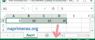
In my opinion, the best way to calculate the sum of absolute values in Excel is to use a helper column. To cell B2

enter the formula:

Then extend it to cell B8

.
ABS
function returns the modulus of a number.
So now we can simply sum the range B2:B8
and that will give us the result.

SUM(B2:B8) =SUM(B2:B8)

In my example the range is A1:A8

is a full-fledged data table.
Therefore, when you added the formula =ABS(A2)
to cell
B2
, Excel expanded the table and automatically filled in all the cells in the column.
Next, I went to the Design tab ,

Table
group of tabs , and checked the box next to the
Total
Row option.
All values in column B
were automatically summed, and the result was displayed in a separate row.

To calculate the amount in the total line, use the SUBTOTAL

(SUBTOTAL).
This is a general-purpose function that can perform sums, just like the SUM
.
But there are also significant differences, for example, SUBTOTAL
completely ignores numbers that were hidden manually or using filtering. There are a few other differences, but these have little to do with the topic of this article.

The good thing about the auxiliary column method is that it gives you more flexibility if you need to use the data in the future, for example, in the form of a table or a pivot table. In addition, the auxiliary column can be used to sort numbers modulo.

This is undoubtedly a very good way, but what to do when you need to fit everything into one formula without any auxiliary columns?