Syntax
=VLOOKUP(item_to_be_found, table_address_where_the_search_value_is_located, column_ordinal_number, interval_lookup)
Element – can be numeric (cell address) or text (“text”).
The table address is the range of cells where the value is approximately located.
Column number – accepts an integer from the range from 1 to n, the result will be extracted from it.
Interval scanning - an approximate (closest) match to the criterion is designated as 1 (true), and an exact match is designated as 0 (false). This Boolean argument is optional if the table is sorted from minimum to maximum value. If the table is not sorted and the argument is omitted, this is equivalent to true.
Important! The value you are looking for must be to the left (in the first column) of the returned element.
In the Russified version of Excel, arguments are entered through the “;” sign, in the English version - through a comma.
Substituting data from one Excel table to another
This action is performed in the same way. For our example, you can not create a separate table, but simply enter a function in a column of any of the tables. Let's show it using the first example. Place the pointer in the last column.
And in cell G3 place the VLOOKUP function. We again take the range from the adjacent sheet.
As a result, the column of the second table will be copied to the first.
That's all the information about the invisible but useful VLOOKUP function in Excel for dummies. We hope it will help you in solving problems.
Errors
When the user makes a mistake when entering data or selecting a range, various errors are displayed instead of the result: #N/A, #VALUE, #REF.
The #N/A error appears if:
- The specified range does not contain the element you are looking for.
- The element you are looking for is less than the minimum in the array.
- An exact search was specified (argument FALSE or 0), but the searched item is not in the range.
- An approximate search was specified (TRUE or 1), but the data is not sorted in ascending order.
- The cell where the search is taken from and the cell with the data in the first column have a different format (numeric and text).
- There are spaces or invisible non-printing characters in the code.
- Time values or large decimal numbers are used.
To avoid the #N/A error, when VLOOKUP does not find the value, it is recommended to use the following formula: =IFERROR(VLOOKUP(C2,A1:B12,2,FALSE),0) – instead of 0, you can write “not found”.
The #VALUE error appears if:
- The column number is 0.
- The first argument is longer than 255 characters.
The #REF error occurs if the third argument is greater than the number of columns in the table.
Video - “Quick data transfer using the VLOOKUP function in Excel”
Transferring data using VLOOKUP can be used not only to quickly obtain data from one table to another, but also to compare two tables.
This is very important for those who work in procurement and send orders to the supplier.
Usually the following situation occurs. You send an order to the supplier, after a while you receive a response in the form of an invoice and compare the order with the invoice.
Is everything on the bill, in the right quantity, at the right prices, etc.
Search and substitution using multiple conditions
45300 01.05.2015
Formulation of the problem
If you are an advanced user of Microsoft Excel, you should be familiar with the VLOOKUP function .
or
VLOOKUP
(if not yet, then read this article first to become one). For those who understand, there is no need to advertise it - not a single complex calculation in Excel can be done without it. There is, however, one problem: this function can only search for data by matching one parameter. What if we have several of them?
Let's assume that we have a database of product prices for different months:
You need to find and pull out the price of a given product ( Nectarine
) in a certain month (
January
), i.e.
get 152
, but automatically, i.e. using the formula. VLOOKUP in its pure form will not help here, but there are several other ways to solve this problem.
Method 1: Additional Search Key Column
This is the most obvious and simple (although not the most convenient) method. Since the standard VLOOKUP
can search only by one column, and not by several, then we need to make one out of several!
Let's add another column next to our table, where we will merge the product name and month into a single whole using the concatenation operator (&) to get a unique key column for searching:
Now you can use the familiar VLOOKUP
to find the glued pair
NectarineJanuary
from cells H3 and J3 in the created key column:
pros
: Simple method, familiar function, works with any data.
Minuses
: It is necessary to create an additional column and then, perhaps, also hide it from the user. When changing the number of rows in the table, extend the concatenation formula to new rows (although this can be simplified by using a smart table).
Method 2. SUMIFS function
If you need to find exactly a number (in our case, the price is just a number), then instead of VLOOKUP you can use the SUMIFS
, which appeared starting in Excel 2007. In theory, this function selects and sums numeric values according to several (up to 127!) conditions. But if our list does not have duplicate products within the same month, then it will simply display the price value for the given product and month:
pros
: No additional column is needed, the solution is easily scaled to a larger number of conditions (up to 127), and calculates quickly.
Minuses
: Works only with numeric output, not applicable for text search, does not work in older versions of Excel (2003 and earlier).
Method 3. Array formula
How to use the INDEX
and
MATCH
as a more powerful alternative to VLOOKUP, I have already described in detail (with video). In our case, we can use them to search across several columns in the form of an array formula. For this:
- Select the empty green cell where the result should be.
- In the formula bar, enter the following formula into it:
- Press at the end not Enter, but the combination Ctrl+Shift+Enter
to enter the formula not as a regular one, but as an array formula.
How it actually works:
The INDEX function returns the contents of the Nth cell in order from the price range C2:C161. In this case, the serial number of the desired cell is found for us by the SEARCH function. She is looking for a combination of product name and month ( NectarineJanuary
) in turn in all cells of the range A2:A161&B2:B161 merged from two columns and gives the serial number of the cell where it found an exact match. Essentially, this is the first method, but the key column is created virtually right inside the formula, and not in the worksheet cells.
pros
: No need for a separate column, works with both numbers and text.
Minuses
: Significantly slows down on large tables (like all array formulas, however), especially if you specify ranges “with a margin” or entire columns at once (i.e. instead of A2:A161 enter A:A, etc.) Formulas are unusual for many array in principle (then come here).
Related links
- How to search and substitute data using the VLOOKUP function
- What are array formulas and how to use them
- How to use a combination of INDEX and MATCH functions instead of VLOOKUP
- How to extract all values at once, not just the first one using VLOOKUP
MCH
21.07.2015 00:27:28
What about SUMPRODUCT:
| =SUMPRODUCT((B2:B161=H3)*(C2:C161=J3)*L3) |
Or an array formula:
| =MIN(IF((B2:B161=H3)*(C2:C161=J3),L3)) |
Where instead of MIN you can use MAX or SUM (if the Product/Month combinations are unique)
Link
Vlad Kulikov
23.07.2015 13:32:15
There is also an option), in case the array is lower or higher, or simply within a certain range. This formula was suggested to me by a person from the forum under the nickname Evgeniy =INDEX($A$1:$D$173;MAX(IF($A$1:$D$173=G3&I3;ROW($A$1:$D$173)));MAX( IF($A$1:$D$173=K2,COLUMN($A$1:$D$173)))) Example from the link below: Parent Link
Nikolay Pavlov
22.08.2015 11:35:56
I completely agree, Mikhail. But you need to remember that these formulas only work for numbers and in the presence of duplicate Product-Month
will sum them up and not return the first value encountered, i.e. this is for summing across two conditions rather than sampling. Parent Link
MCH
23.08.2015 09:29:36
The example with SUMPRODUCT() works in the same way as the above “Method 2” with SUMIFS() with the same restrictions (it works with numbers and unique product/month combinations are required, otherwise we will get the sum), but there is also an advantage - it works in Excel 2003. I gave these examples as additional “sampling” options. Well, another option via VIEW:
| =VIEW(2,1/(A2:A161=G3)/(B2:B161=I3),C2:C161) |
Among the advantages - it does not require massive input, works in any version of Excel, you do not need to do concatenation as in the example with VLOOKUP, it works significantly faster than the design with INDEX (MATCH) when using zero interval lookup (exact search). Feature - if there are several product/month combinations that fall under the selection, it will return the value of the last match. An analogue of this formula through INDEX (SEARCH):
| =INDEX(C2:C161,MATCH(2,1/(A2:A161=G3)/(B2:B161=I3))) |
Requires massive input and will return the last match. For the first match:
| =INDEX(C2:C161,MATCH(1,(A2:A161=G3)*(B2:B161=I3),0)) |
But on a large amount of data, this formula will work significantly slower than the previous two options.
Parent Link
Elena Red
07.02.2017 17:12:53
=MIN(IF((B2:B161=H3)*(C2:C161=J3);L3)) Where does the variable “L3” come from in the formula if it needs to be calculated?? Parent Link
ILYA_
24.07.2015 13:09:52
Hello Nikolay!
I often use method 1. We have to analyze information on different days and for different, uneven periods of time. In order to have objective information, I convert the date and time into something like this: 03/25/2015 2:39:48 = 25_3_2015_2_39_48, then I pull out the VLOOKUP values, put the formula =ND() in the empty cells and build a graph.
Link
Alexey St.
25.07.2015 22:02:52
Greetings Nikolay! Do you have any plans to create a video lesson on the topic of “what if” analysis? Link
vikttur
01.09.2015 16:34:39
another option: = AVERAGEIFS(C:C;A:A;G3;B:B;I3) accordingly, when duplicating rows, it will give their average. Nikolay such a question, how do you select a function without a mouse and its completion? in the video in typed “=in” and pressed something (time 8:55), and immediately “=Index(” Link appeared
Vasily Alibabaevich
23.10.2015 11:11:55
I didn’t see the video... but I pressed TAB Parent Link
Zoynels
18.09.2015 16:52:30
I often use a combination of all three options, only using IndexID=string() as the key. Then I sum up the IndexID column according to the condition, and through INDEX I find the required column. The formula is:
| =INDEX(Price[Price],SUMSLIMS(Price[IndexID],Price[Product],H3,Price[Month],J3),1)). |
And for the second option, you can eliminate repetitions using the formula:
| =IFERROR(SUMIFS(C:C,A:A,G3,B:B,I3)/COUNTIFS(A:A,G3,B:B,I3) “Nothing found!”) |
which will first sum all the found values and then divide by their number. You just need to keep in mind that you can’t divide by zero/
Link
talot
25.11.2015 12:01:55
| And for the second option, you can eliminate repetitions using the formula: =IFERROR(SUMIFS(C:C,A:A,G3,B:B,I3)/COUNTIFS(A:A,G3,B:B,I3);"Nothing found!";) |
Why not use the AVERAGEIFS() function for this? AVERAGEIFS(C:C;A:A;G3;B:B;I3) and that’s it.
Parent Link
IgorF
02.12.2015 17:54:05
Nikolay, for the 3rd case you can make a formula very similar to yours, but without using an array: =INDEX(C:C;SEARCH(G3&I3;INDEX(A:A&B:B;0);0)) =INDEX(C :C;MATCH(G3&I3;INDEX(A:A&B:B;0);0)) If you enter 0 as the second parameter in the index function, then it is processed as an array Link
Nikolay Pavlov
06.12.2015 14:32:57
Thank you for sharing, Igor - a very valuable clarification. Parent Link
Natalia
22.09.2016 11:13:45
Igor, please tell me, if in the combination of columns A and B the formula does not find the combination G3&I3, how can I make the result in the cell be “0”... I try your formula, and in this case “#N/A” appears in the cell.... Thanks in advance.. Parent Link
IgorF
22.09.2016 11:16:48
Natalya, use the function =IFERROR(INDEX(C:C;MATCH(G3&I3;INDEX(A:A&B:B;0),0));0) =IFERROR(INDEX(C:C;MATCH(G3&I3;INDEX(A :A&B:B;0);0));0) Parent Link
Natalia
22.09.2016 11:37:06
Hurray!!!! It worked... Thanks a lot! Parent Link
Trofim Kozhemyakin
21.05.2018 19:05:28
Igor and Nikolay, thank you very much! For some reason the array formula didn't work. The formula contained references to columns, but the name of the smart table was not reflected. The formula without using an array worked. Parent Link
Igor Yakovlev
08.12.2015 12:55:09
How to calculate the amount by a certain date. For example, there are dates in the 1st column (always different) and amounts in the second. You need to calculate what amount comes out on the 25th of each month. Example: Date Paid Issued invoice 12/30/13 15,000 rub. 01/02/14 12,000 rub. 01/15/14 16000 rubles 01/31/14 45000 rubles 02/05/14 50000 rubles 02/08/14 65000 rubles 02/12/14 1000 rubles 02/25/14 12000 rubles 02/28/14 20000 rubles 03/03/14 120 00 rub 03/21/14 17000 rub 05/24/14 40000 rub 05/24/14 20,000 rubles You need to know the debt on the 25th of each month. Help me please. Link
Ulyana Maksimova
08.05.2016 00:57:14
Hello, please help: is it necessary to automatically select the planning month (January or February, etc.) if there is a value in this month? Thanks Link
Natalia
22.09.2016 00:08:18
Nikolay, good afternoon! I tried to use method No. 3, it is the most suitable for me, but I couldn’t apply the formula, it gives an error (#VALUE!)... I created an analogue of your example, but the formula continues to give an error... I don’t understand what the problem is:| Link
Anna
11.01.2017 14:42:21
Natalya, are you sure you put the curly braces in the array after writing the formula? (Ctrl+shift+Enter). Also check the condition column formats. Everything works. Thank you very much for the formula) Parent Link
Kirill Gibizov
23.01.2017 18:11:04
Thank you, Nikolay. Thanks Igor. Everything worked great. Life has become easier, life has become more fun! =) Link
Dmitry Boltyansky
26.02.2017 20:39:30
+1. Just thank you. Otherwise, I was “sure that VLOOKUP is the most complex function in Excel, and I’ve already mastered it, which means it won’t teach me anything new.” Link
Volk
03.04.2017 19:45:31
But if the pillars are not nearby, is it possible to glue them together? 1
| criterion1 | value | value | value | criterion 2 | value | what we are looking for |
| auto | 1 | er | er | 11 | ahh | text |
| auto | 1 | here | here | 11 | up | text |
| moto | 2 | er | er | 22 | up | text |
| moto | 2 | re | eyer | 22 | uptap | text |
Link
Volk
03.04.2017 19:59:33
Tell me how to make VLOOKUP look only at visible cells in a filtered table and substitute them into another filtered table? Link
Pavel Minaev
07.06.2017 13:40:38
Please tell me. !!! I just can’t beat the calculation of the formula with INDEX and MATCH... using the first parameter. The task is this... There are a number of parameters - using them in the data array you need to find a match based on 2 or more matches. Moreover, the first parameter is repeated and located in a column, the second one changes and is located in a row. MATCH - finds the first match using the first parameter, and ignores the second match... Link
Ali
22.06.2017 02:18:46
Good afternoon. I have a slightly different task. There is a “Sales” page in which, when filling out the product and the date of sale, the recommended price from the “Prices” page should be inserted. At the same time, on the “Prices” page the same product can appear several times (if it was purchased more than once and the purchase price was different). Also, on the “Prices” page, each product indicates the price setting date, which coincides with the posting date. I need the last price to be set. The option in which in the “Prices” section the purchase price will change dynamically when a new batch of goods arrives does not suit me, because in this case, the profit data for previously sold goods will constantly change, which will be an error. The algorithm for how price substitution should look is generally clear to me, but I can’t figure out what the formula should look like. The algorithm (as it seems to me) should be as follows: Take the sales date and look for the closest (earliest) price setting date from the “Prices” page for the selected product, and pull out the price. Of course, I understand that 1C is needed for this purpose, but my friend (who asked me to write this table) cannot enter his products into the common database. Help me please. Data on prices must be taken from columns I, J, K (page “Prices”;) and substituted into columns J, K, L (page “Sales”). Example from the link: Example Link
passion fruit
23.08.2017 16:01:55
Wouldn't this option suit you: filter the list of prices by sale date, starting with the latest (descending)? VLOOKUP will select the very first value, i.e. top. That. if you have a filter by date, then the function will find the most recent price. Further, the principle of searching for a price is the same as in the article... Parent Link
passion fruit
23.08.2017 14:11:18
Hi all! Please tell me how you can show in one line in which months, for example, potatoes were sold? What formula should you use? Is it even possible to do this using standard formulas without additional macros? In my case, I need to display all the sizes that are available for one shoe article in ONE LINE (column shoe article, column shoe size). Link
Vladimir Butyrirn
01.06.2018 11:53:00
The array formula helped, the first two options do not solve more complex problems than in the examples. Thank you! Link
Irina Irina
24.08.2018 14:26:12
Good afternoon Help, please, I seem to be doing something wrong at some stage. There is a list linking phone number - position, there is also a table linking position - tariff, so I need to link phone-position-tariff. index _searchpoz I am doing the wrong value. Help, please.. thanks Link
sp a
27.11.2018 16:08:39
Good afternoon Tell me, is it possible to use the formula in the 3rd example when searching in different books? Link
Alexander Z
26.09.2019 09:04:55
help me how to write this in Excel B1=C1 B2=C2 if B3< B1 then B3=0 if B3 if B3 ≥B2 then B3=C2 Link
Daria Gaidukova
28.05.2020 14:22:10
Good afternoon Please help me if I need to search not by a single word, but by a phrase (one cell), the first word of which is in one column (select from the text), and the second in the second. I've racked my brain, nothing comes out Link
Anna Matushkina
01.10.2020 13:07:59
What if the conditions are dates and you need to remove the name if it falls inside the range condition between 2 dates? Link