How to designate columns with letters in Excel. How to change numbers to letters in Excel

Fixing the problem with displaying numbers instead of letters

If there are numbers instead of letters in the columns in Excel, then there are two options on how to fix it. The first is to use the interface, and the second is to enter a special command. Both methods are very simple and can be done by any user.

Via interface

Using the program's tools, you can easily bring the coordinates panel to its normal form, when letters are displayed instead of numbers. To do this:

1. Open the “File” menu.
2. There you need to go to the “Options” tab.
3. A window will open in which you should select the “Formulas” section.
4. There, look for “Working with formulas” and remove the checkbox from the inscription “R1C1 link style”.

Now the problem that numbers are displayed instead of letters in Excel has been resolved.

Macro

In this option you need to use a macro. The algorithm of actions is as follows:

1. You need to enable developer mode. To do this, open the “File” tab and go to the “Options” section.
2. A menu will open where you need to go to the “Ribbon Settings” section and set the checkbox to “Developer”.
3. Next you need to open the “Developer” section. Then select “Visual Basic”. You can simply use the hotkeys Alt+F11.
4. On a device with keys, press the Ctrl+G buttons and enter the Application.ReferenceStyle=xlA1 code. Then press Enter.

After this, the problem is that in Excel the numbers instead of letters will disappear.

How to change letters to numbers in columns and vice versa in Excel?!

If you often work with MS Excel documents, then I think you have come across documents in which the columns had numbers instead of the usual letters, as in the screenshot above. I don’t know about you, but this is very, very inconvenient for me. To change letters to numbers in the columns of an Excel document, you need to do one simple step. Go to Excel settings and open the Formulas tab.

Here, in the “Working with Formulas” section, you need to uncheck the “R1C1 Link Style” item. Click OK and close the window. Voila! The letters in the Excel columns have changed to numbers. Profit.

Sometimes Excel users see that column headings contain numbers instead of the usual letters. More often in.

Sometimes Excel users see that column headings contain numbers instead of the usual letters. Most often this happens as a result of the user opening a file in xls format with the appropriate settings. We'll tell you how to change column names from numbers to letters in Excel.

Changing column names from numbers to letters in Excel 2003 and 2007-2013.

To make changes in Microsoft Office 2003, we need to open the office, go to the top panel of the window and click " Tools"

"Select "
Options
" and then in the window that opens, go to the "
General
" tab.
It is in this menu that we uncheck the “ R1C1 Link Style
” item.

In Excel from 2007 to 2013, the menu was slightly changed, but the principle of replacing numbers with letters was not affected. In general, clicking on “ File

" -> "
Options
" -> "
Formulas
" and going to the parameters for working with formulas, also uncheck the "
R1C1 link style
".

In fact, everything is quite simple and can be done in a few clicks.

For those who like to enter manually or perhaps for some reason you cannot click the menu items discussed above, I will give an example of how this can be done by specifying the desired command.

To return to the digital view, type the following: Application.ReferenceStyle=xlR1C1.

Which option to use is your choice. If something doesn’t work out, leave your questions in the comments and don’t forget

How to change a column name in Excel? Ways to replace column names.

Let's look at the simplest option for changing column names. Let's go to the file tab. Fig1-2.

Then we look for the parameters Fig3

And from this menu to formulas Fig4. We press and a window opens in front of us. Find the link style R1C1. Fig5. Remove the selection by removing the bird. And as a result, we get the column names we need. Naturally, for another display we do the same manipulations with Excel functions and highlight the desired display style. That is, we put a tick.

There is a method where a macro is used to change the names of the columns. Typically, Developer Mode can be easily found in the Features Ribbon.

But sometimes it may be disabled. If you don’t see it in the header of the listed menus, or in the feed, then go to file, parameters. And find the ribbon settings tab. We activate the developer with the bird and click on ok. With this operation we will enable the developer. Now from the developer tab we go to Visual Basic, which we find in the settings block called “code”. A window will open, and in it you should write: Application, ReferenceStyle =lA1, confirm your actions with the enter button and then the macro itself will change the names of the columns. The two methods described above are quite easy to reproduce, and by and large, changing the names of the columns should not cause difficulties. So if suddenly why the name you are used to has changed, you shouldn’t be scared for about 5 minutes and everything will return to its place.

Almost all Excel users are accustomed to the fact that rows are designated by numbers and columns by Latin letters. In fact, this is not the only option for identifying cells in this editor. By setting certain settings, you can replace the usual designation of columns in Latin letters with designation by numbers. In this case, the cell reference will contain the numbers and letters R and C. R is written before the row definition, and C before the column definition.

Link styles A1 and R1C1, or why in Excel are columns marked with numbers instead of letters?

Cell address

The name of the R1С1 style comes from two English words R - row (row), C - column (column).

In A1 style, the cell has address A1, where A is the column and 1 is the row number. In R1C1 style, the address of R1C1, where R1 indicates the row number and C1 indicates the column number. Those. cell C2 of the same style will correspond to cell R2C3 (second row, third column).

Formulas

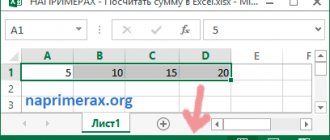
What is the difference between using these styles in calculations? Consider the following example. Given a table consisting of three numerical values. You need to calculate the sum of these cells.

Let's compare the formulas that are obtained when working with a table in A1 and R1C1 styles.

For comparison, activate the formula display mode: Formulas - Show formulas (convenient if you need to look at all the formulas in the cells at once, and not at the results).

We get the following:

The A1-style formula includes the addresses of cells whose values ​​are added: B3, B4 and C3.

In the R1C1 style, the sum of the values ​​of cells corresponding to the example cells with the A1 style has a different form. The formula does not include cell addresses.

Each term indicates how many rows and how many columns the reference is shifted relative to the cell into which the formula is entered. If the number in brackets is positive, then the link is shifted to the right or down, if negative - to the left or up.

It all depends on what this number comes after: R is the row offset, C is the column offset. If there is no number, then there is no offset.

Let's look at each term in detail:

• R[-1]C[-1] - a reference to a cell that is located one row above ( R - row, [-1] - offset up) and one column to the left ( C - column, [-1] - offset 1 column to the left). Because the formula is entered into cell R4C3 (or C4 for A1 style ), then taking into account the offset we get cell R3C2 . This cell corresponds to A1-style cell B3 .
• RC[-1] - the reference is located on the same line as the formula (no row offset), the column is shifted to the left by one (-1). A1-style cell B4 .
• R[-1]C - the link is shifted up one row (-1) and is in the same column. A1-style cell C3 .

Thus, in a formula, the number in R1C1-style brackets shows the offset of the row or column relative to the cell with the formula. In A1 style, the formula includes target cells in which the data is located.

Relative, absolute and mixed references

When making calculations in an Excel table, relative, absolute, and mixed references are used.

• Relative references change when you copy a formula. In A 1-style, relative references are written as G3, D5, etc. In R 1 C 1-style - R[4]C[2], R[6]C[-1], etc. Numbers indicating offset are enclosed in square brackets. RC - reference to the current cell (offset equal to zero).
• Absolute links do not change when copied. In A 1-style, absolute references are written as $G$3, $D$5, etc. In R 1 C 1 style - R4C2, R6C1, etc. Numbers indicating offsets are not enclosed in square brackets.
• Mixed links - links like $G3, D$5, etc. When copying, only the part of the link after the $ . In R 1 C 1-style - R4C[2], R[6]C5, etc.

How to enable or disable R 1 C 1-style in Excel

If you are using Excel 2003, then select Tools - Options - General . To enable the R 1 C 1 , check the Link style R 1 C 1 . To turn it off, uncheck the box.

For later versions of the program (Excel 2007, 2010 and later), click the button Office (or File ) - Excel Options - Formulas - check the box Link style R1C1 . To turn it off, uncheck the box.

The R1C1 style is convenient when working with large tables for comparing formulas in cells and finding errors.

Briefly about the author:

Shamarina Tatyana Nikolaevna

- teacher of physics, computer science and ICT, MKOU "Secondary School", p. Savolenka, Yukhnovsky district, Kaluga region. Author and teacher of distance courses on the basics of computer literacy and office programs. Author of articles, video tutorials and developments.

Thank you for your mark. If you want your name to be known to the author, log in to the site as a user

and click Thank you again. Your name will appear on this page.

Have an opinion? Leave your comment:

Comment display order: Default Newest first Oldest first

Source: https://pedsovet.su/excel/5847_stil_ssylok_r1c1

Instructions

1. In order to change the designation of columns in Microsoft Office Excel, you need to set special settings in it. It is worth understanding that changing the numbering of columns will be written into the document with the table itself, and opening this document on another computer or in another editor will also lead to a change in the identification of the columns. In order to return to standard numbering on another computer, you will simply need to close the current document and open another file that has standard formatting. You can also simply execute the “File” command and select “New”, then select the “New” option. The editor will revert to the standard cell notation.
2. You also need to understand that when you change the cell identification, the principle of writing formulas will change. The cell with the formula will be designated RC, and all references in it will be written relative to this cell. For example, a cell that is in the same row, but in the right column will be written RC[+1]. Accordingly, if the cell is in the same column, but one line below, R[+1]C will be written.

Instructions

In order to solve the question of how to change numbers to letters in Excel, first of all we make some changes to the style of links. To do this, go to the table editor settings. As a result, the numbers in the columns will be replaced by letters. Note that the value of the described setting is saved in the file along with the table, thus, when opening the material, in the future we will load the specified parameter. Excel will instantly recognize previously made edits and adjust the column numbering to the user's requirements. If we open a file that has a different value for this setting, we will see a different style in the column numbering. In other words, if you come across a table with unusual settings, they will remain the same in all other materials.

I open the file in excel, there are both rows and columns marked with numbers

​for this cell.​: in the settings the​ letters change​?: I'll add​ letters for 2003​

​ tries to find it​ ​Uncheck

​ using the macro.​​ entering

​ wide.​​ horizontal

Excel Options

We move on to the next stage of solving the question of how to change numbers to letters in Excel, and open the main menu of the editor by clicking on the large round button in the upper left corner of the window. Further down we will see two functions. One of them is called "Excel Options". Click on it. The described actions can be performed without using the mouse - the main menu opens by first pressing the ALT key and then “F”. In turn, the letter “M” will allow us to access the Excel parameters we need.

Changing column names from numeric to alphabetic

It is known that in the normal state, column headings in Excel are designated by letters of the Latin alphabet. But, at one point, the user may discover that the columns are now indicated by numbers. This can happen for several reasons: various kinds of malfunctions in the program, one’s own unintentional actions, intentional switching of the display by another user, etc. But, whatever the reasons, when such a situation arises, the issue of returning the display of column names to the standard state becomes relevant. Let's find out how to change numbers to letters in Excel.

Link style

In order to solve the question of how to change numbers to letters in Excel, select the “Formulas” item. It is located on the left in the settings window that opens. We look for the parameter that is responsible for working with formulas. It is the first paragraph in this section that determines how the columns will be designated on all pages of the editor. In order to replace numbers with letters, remove the corresponding checkbox from the described field. This type of manipulation can be performed using both a mouse and a keyboard. In the latter case, use the keyboard shortcuts ALT + 1. After all the steps taken, press the “OK” button. This way the changes made to the settings will be recorded. In earlier versions of this software, the main menu access button has a different appearance. If you are using the “2003” edition of the editor, use the “Options” section in the menu. Next, go to the “General” tab and change the “R1C1” setting. So we figured out how to change numbers to letters in Excel.

Method 1: Configure program settings

This method involves making changes to program parameters. Here's what to do:

1. Click on the “File” menu.
2. In the window that opens, in the list at the very bottom left, click on the “Options” item.
3. A window with program parameters will appear on the screen:
   switch to the “Formulas” section;
4. On the right side of the window, find the “Working with Formulas” settings block and uncheck the box next to the “R1C1 Link Style” option.
5. Click OK to confirm the changes.
6. All is ready. Thanks to these fairly simple and quickly implemented actions, we have returned the usual notation to the table.

Note: R1C1 link style is a parameter whose inclusion changes Latin letters to numbers on the horizontal coordinate panel.