Instructions on how to work with tables in Excel (in simple words)

How to work with tables in Excel. Step-by-step instruction

Before working with tables in Excel, follow these recommendations for organizing data:

• Data should be organized in rows and columns, with each row containing information about one record, such as an order;
• The first row of the table should contain short, unique headings;
• Each column must contain one type of data, such as numbers, currency, or text;
• Each row should contain data for one record, such as an order. If applicable, provide a unique identifier for each line, such as an order number;
• The table should not have empty rows and absolutely empty columns.

Select an area of ​​cells to create a table

Select the area of ​​cells in which you want to create a table. Cells can be either empty or with information.

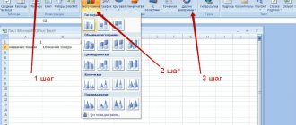
Click the Table button on the Quick Access Toolbar

On the Insert tab, click the Table button.

Select cell range

In the pop-up, you can adjust the location of the data and also customize the display of headings. When everything is ready, click “OK”.

The table is ready. Fill in the data!

Congratulations, your table is ready to be filled out! You will learn about the main features of working with smart tables below.

Video lesson: how to create a simple table in Excel

Formula 7: LEVSIMV

This function makes it possible to select the required number of characters from the left of the line.

Its syntax is as follows:

=LEFT(text,[number_characters])

Possible arguments:

1. Text is a string from which you want to extract a certain fragment.
2. Number of characters – directly the number of characters that need to be extracted.

So, in this example you can see how this function is used to see what the appearance of titles for website pages will be. That is, whether the string will fit into a certain number of characters or not.

Formatting a table in Excel

Pre-configured styles are available to customize the table format in Excel. All of them are located on the “Design” tab in the “Table Styles” section:

If 7 styles are not enough for you to choose from, then by clicking on the button in the lower right corner of table styles, all available styles will open. In addition to the styles preset by the system, you can customize your format.

In addition to the color scheme, in the table “Designer” menu you can configure:

• Show header row – enables or disables headers in the table;
• Total line – enables or disables the line with the sum of the values ​​in the columns;
• Alternating lines – highlights alternating lines with color;
• First column – makes the text in the first column with data “bold”;
• Last Column – makes the text in the last column “bold”;
• Alternating columns – highlights alternating columns with color;
• Filter Button – Adds and removes filter buttons to column headers.

Video lesson: how to set the table format

conclusions

Of course, these are not all the functions that are used in Excel. We wanted to present ones that the average spreadsheet user has not heard of or rarely uses. In statistics, the most commonly used functions are to calculate and average. But Excel is more of a development environment than just a spreadsheet program. It can automate absolutely any function.

I really hope that it worked out and that you learned a lot of useful things for yourself.
Rate the quality of the article. Your opinion is important to us:

How to add a row or column to an Excel table

Even within an already created table, you can add rows or columns. To do this, right-click on any cell to open a pop-up window:

• Select “Insert” and left-click on “Table Columns on the Left” if you want to add a column, or “Table Rows Above” if you want to insert a row.

• If you want to delete a row or column in a table, then go down the list in the pop-up window to the “Delete” item and select “Table Columns” if you want to delete a column or “Table Rows” if you want to delete a row.

Quickly jump to the desired sheet

If the number of worksheets in a file exceeds 10, then it becomes difficult to navigate through them. Right-click on any of the sheet tab scroll buttons in the lower left corner of the screen. A table of contents will appear, and you can go to any desired sheet instantly.

How to filter data in an Excel table

To filter information in the table, click the arrow to the right of the column heading, after which a pop-up window will appear:

• “Text filter” is displayed when there are text values ​​among the column data;
• “Filter by color”, just like a text filter, is available when the table has cells painted in a color different from the standard design;
• “Numerical filter” allows you to select data by parameters: “Equal to...”, “Not equal to...”, “Greater than...”, “Greater than or equal to...”, “Less than...”, “Less than or equal to...”, “Between...”, “Top 10...”, “Above average”, “Below average”, and also set up your own filter.
• In the pop-up window, under “Search”, all data is displayed, by which you can filter, and with one click, select all values ​​or select only empty cells.

If you want to cancel all filtering settings you have created, open the pop-up window above the desired column again and click “Remove filter from column”. After this, the table will return to its original form.

Formula 2: If

This function is necessary if the user wants to specify a certain condition under which a calculation should be carried out or a specific value should be output. It can take two options: true and false.

Syntax

The formula for this function has three main arguments and looks like this:

=IF(logical_expression, “value_if_true”, “value_if_false”).

Here, a logical expression means a formula that directly describes the criterion. With its help, data will be checked for compliance with a certain condition. Accordingly, the “value if false” argument is intended for the same task, with the only difference that it is the mirror opposite in meaning. In simple words, if the condition is not confirmed, then the program performs certain actions.

There is another option for using the IF

– nested functions. There can be many more conditions here, up to 64. An example of reasoning corresponding to the formula shown in the screenshot is as follows. If cell A2 is equal to two, then you need to output the value “Yes”. If it has a different value, then you need to check whether cell D2 is equal to two. If yes, then you need to return the value “no”; if here the condition turns out to be false, then the formula should return the value “possibly”.

It is not recommended to use nested functions too often, since they are quite difficult to use and errors may occur. And it will take a lot of time to fix them.

IF function

can also be used to understand whether a certain cell is empty.
To achieve this goal, you need to use one more function - EMPTY
.

Here the syntax is as follows:

=IF(EMPTY (cell number), “Empty”, “Not empty”).

In addition, it is possible to use EMPTY

apply the standard formula, but specify that the condition is that there are no values ​​in the cell.

IF -

This is one of the most common functions that is very easy to use and it makes it possible to understand how true certain values ​​are, get results based on various criteria, and also determine whether a certain cell is empty.

This function is the foundation for several other formulas. We will now analyze some of them in more detail.

How to fix a table header in Excel

The tables you have to work with are often large and contain dozens of rows. Scrolling down a table makes it difficult to navigate the data if the column headings are not visible. In Excel, you can attach a header to a table so that when you scroll through the data, you will see the column headings.

To fix headers, do the following:

• Go to the “View” tab in the toolbar and select “Freeze Panes”:

• Select “Freeze top row”:

• Now, when scrolling through the table, you will not lose the headers and can easily find out where the data is located:

Video lesson: how to attach a table header:

Formula 8: PSTR

This function makes it possible to get the required number of characters from the text, starting with a certain character in a row.

Its syntax is as follows:

=PSTR(text, initial_position, number_of_characters).

Decoding the arguments:

1. Text is a string that contains the required data.
2. The starting position is the actual position of the character that serves as the beginning for text extraction.
3. Number of characters – the number of characters that the formula should extract from the text.

In practice, this function can be used, for example, to simplify the names of titles by removing words that appear at the beginning of them.

How to flip a table in Excel

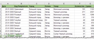
Let's imagine that we have a ready-made table with sales data by manager:

On the table at the top, the names of the sellers are indicated in the rows, and the months in the columns. In order to turn the table over and place the months in the rows, and the last names of the sellers, you need:

• Select the entire table (hold down the left mouse button to select all table cells) and copy the data (CTRL+C):

• Move the mouse cursor to a free cell and press the right mouse button. In the menu that opens, select “Paste Special” and left-click on this item:

• In the window that opens, in the “Insert” section, select “values” and check the “transpose” box:

• Ready! Months are now placed in rows, and seller names in columns. All that remains to be done is to convert the received data into a table.

Learn Excel Basics: Cells and Numbers

Note: all screenshots below are from Excel 2016 (as one of the newest ones today).

Many novice users, after launching Excel, ask one strange question: “well, where is the table?” Meanwhile, all the cells that you see after starting the program are one big table !

Now to the main thing: any cell can contain text, some number, or a formula. For example, the screenshot below shows one illustrative example:

• left: cell (A1) contains the prime number “6”. Please note that when you select this cell, the formula bar (Fx) simply shows the number “6”.
• on the right: in cell (C1) there is also a simple number “6”, but if you select this cell, you will see the formula “=3+3” - this is an important feature in Excel!

Just a number (on the left) and a calculated formula (on the right)