New Sheet button
See also: “Hotkeys in Excel”
Of course, this is the easiest and most accessible method, which is most likely used by the majority of users of the program. It's all about the maximum simplicity of the adding procedure - you just need to click on the special “New Sheet” button (in the form of a plus), which is located to the right of the existing sheets at the bottom of the program window.
The new sheet will be named automatically. To change it, you need to double-click on it with the left mouse button, write the desired name, and then press Enter.
Insertion Methods
A new sheet can be added in four ways, which are suitable for all versions of the editor, including programs released in 2003, 2007, 2010, and 2020.
- 1. Press the special button, which is located to the right of the last tab in the list.
In later versions, instead of such a button there is a regular plus sign in a circle.
- 2. On the main tab of the Toolbar, in the Cells block, look for Insert. Click and at the end of the drop-down list select the desired line.
- 3. Right-click on the shortcut and select Paste from the list. A special window will appear in which you can select not only a sheet, but also a diagram, template or macro.
- 4. The last method is the fastest. Just press the Shift+F11 hotkeys on your keyboard.
On a note! This combination also appears in tooltips when using the previous methods.
It is worth mentioning separately about inserting a worksheet from another file. Right-click on any shortcut and select the Move/Copy line.
A small window will appear in which you need to select the excel workbook and insertion location. Be sure to check the copy box if you are copying a worksheet. Finally, confirm the action with the OK button. The selected label with all the information will be duplicated in another book.
How to add a sheet through the program ribbon
Of course, the function of adding a new sheet can also be found among the tools located in the Excel program ribbon.
- Go to the “Home” tab, click on the “Cells” tool, then click on the small down arrow next to the “Insert” button.
- It’s easy to guess what you need to select from the list that appears - this is the “Insert Sheet” item.
- That's all, a new sheet has been added to the document
Note: in some cases, if the size of the program window is sufficiently stretched, there is no need to look for the “Cells” tool, because the “Insert” button is immediately displayed in the “Home” tab.
Excel doesn't have sheets, what should I do?
Sometimes, users encounter such a problem that at the bottom of the Excel window, where all sheets should be listed, there is simply no panel (only a horizontal scroll bar). In this case, do not worry, this is not a file or program error, but simply specific settings. And now we’ll look at how to indicate them correctly.
In Excel 2003 . Open “Tools” in the top menu, then select “Options”. Make sure you're in the View tab, then check the Show Sheet Labels box.
In Excel 2007 . Open the main menu button (top left), then click Excel Options. Go to "Advanced" and then check the "Show sheet shortcuts" box.
In Excel 2010, 2013, 2016 . Expand the File menu and select Options. Go to “Advanced” and check the box next to “Show sheet shortcuts”.
After this, the sheet pane on the bottom left side should appear.
If you know other useful methods, feel free to share them in the comments.
☕ Would you like to express your gratitude to the author? Share with your friends!
- How to make a link in Word?
- How to save a picture from Word to jpg?
- How to make a link in Word? Word, Excel, OpenOffice
- How to merge cells in Excel? Word, Excel, OpenOffice
- How to make an em dash in Word? Word, Excel, OpenOffice
- How to save a picture from Word to jpg? Word, Excel, OpenOffice
- How to create a page break in Word? Word, Excel, OpenOffice
- How to make a fraction in Word? Word, Excel, OpenOffice
Loading from EXCEL to 1C. List of EXCEL sheets
This article provides functionality with which the processing of “Import from EXCEL and other sources (xls, xlsx, ods, sxc, dbf, mxl, csv, sql) in 1C” : //infostart.ru/public/120961 is performed reading data from table type files *xls, *.xlsx, *.ods, *.sxc. Methods for downloading from an external source: - “MS ADO” method (Reading xls, xlsx files using Microsoft ADO): //infostart.ru/public/163640/ - “MS EXCEL” method (Reading xls, xlsx files with pictures using Microsoft Office ): //infostart.ru/public/163641/ - Method "LO CALC" (Reading xls, xlsx, ods, sxc files with pictures using LibreOffice): //infostart.ru/public/163642/ - Method "NativeXLSX" ( Reading xlsx files with pictures using 1C.BuilderDOM): //infostart.ru/public/300092/ - Method “NativeXLSX”. Previous option (Reading xlsx files using 1C. Reading XML)://infostart.ru/public/225624/ - Method “Excel1C” (Download on platform 8.3.6 with pictures. Reading xls, xlsx, ods files): //infostart. ru/public/341855/ — List of sheets of the file: //infostart.ru/public/163724/
There are many publications on the topic of loading from EXCEL, but “Do you need a ticket taker? - I needed it, but they already took it. - Maybe I’ll be good for something? “Maybe you’ll do well if you don’t show your teeth…” “THE ELUSIVE AVENGERS” (1966).
// The function returns a list of values containing the names of the sheets of the EXCEL book or an Empty List of Values. //// Parameters:// FileEXCEL - Full file name (path to the file with file name and extension). // ConnectionADODB - ADODB driver type for connecting to EXCEL.//// Return values:// SheetList - List of sheet names in the file, for example: Sheet1, Sheet2, Sheet3. //Function FileExcelGetSheetList(Value FileEXCEL, Value ConnectionADODB = "MicrosoftJetOLEDB40") Variable SheetList, TotalSheets, SheetName, SheetArray ; Variable ServiceManager, Desktop, Properties1, Properties2, Arguments, Book, Sheets; Variable ConnectionString, ADODBConnection, ADOXCatalog; SheetList = New ValueList; File = New File(FileEXCEL); If VReg(File.Extension) = ".ODS" OR VReg(File.Extension) = ".SXC" Then // For files of type .ODS,*.SXC we use ServiceManager LibreOffice. Attempt // Initializing the main COM object of type com.sun.star.ServiceManager (LibreOffice/OpenOffice). ServiceManager = New COMObject("com.sun.star.ServiceManager"); // Initialize the child Desktop object. Desktop = ServiceManager.CreateInstance("com.sun.star.frame.Desktop"); // Declaration of properties and arguments for creating an object of type EXCEL Book. Properties1 = ServiceManager.Bridge_GetStruct("com.sun.star.beans.PropertyValue"); Properties1.Name = "AsFile"; // Property “AS FILE”, alternative to “AsTemplate” - “AS TEMPLATE”. Properties1.Value = True; Properties2 = ServiceManager.Bridge_GetStruct("com.sun.star.beans.PropertyValue"); Properties2.Name = "Hidden"; // Run stealthily. Implemented in LibreOffice 3.6. Properties2.Value = True; Arguments = New COMSafeArray("VT_VARIANT", 2); Arguments.SetValue(0, Properties1); Arguments.SetValue(1, Properties2); // Desktop child object: EXCEL Book. Book = Desktop.LoadComponentFromURL(ConvertToURL(FileEXCEL), "_blank", 0, Arguments); // Child object of Book: EXCEL sheets. Sheets= Book.getSheets(); TotalSheets = Sheets.getCount(); // Formation of a list of sheets of the file. For it = 0 BY TotalSheets -1 Loop SheetName = Sheets.getByIndex(it).Name; SheetList.Add(SheetName); // Add the sheet name to the list without a sign. EndCycle; // Shut down. // Closing Objects. Book.Close(True); Desktop.Terminate(); Desktop = Undefined; ServiceManager = Undefined; Exception Report(NStr("ru = '"+ErrorDescription()+"'"), MessageStatus.Attention); Return New ValueList; // In case of error, return an empty list of values. EndAttempt; Otherwise // For files of type .XLS .XLSX we use MS ADODB. // Connection string - definition of the driver that will be used to connect to the EXCEL file. If ConnectionADODB = "MicrosoftACEOLEDB12" Then // ACE.OLEDB.12.0 - To use this connection, additional software is required: // Microsoft Access Database Engine 2010 Redistributable 32/64 bit. ConnectionString = "Provider=Microsoft.ACE.OLEDB.12.0;Data Source= " + AbbrLP(FileEXCEL) + ";Extended Properties=""Excel 12.0;HDR=YES;IMEX=1;"""; // Another option. //ConnectionString = "Driver={Microsoft Excel Driver (*.xls, *.xlsx, *.xlsm, *.xlsb)};Dbq=" + Abbr(FileEXCEL) + ";"; Otherwise // Jet.OLEDB.4.0 - Standard connection, which, as a rule, does not require the installation of additional software. // It is recommended to install the latest Windows Service Pack. ConnectionString = "Provider=Microsoft.Jet.OLEDB.4.0;Data Source= " + AbbrLP(FileEXCEL) + ";Extended Properties=""Excel 8.0;HDR=YES;IMEX=1;"""; // Another option. //ConnectionString = "Driver={Microsoft Excel Driver (*.xls)};Dbq=" + Abbreviation(EXCEL File) + ";"; endIf; Trying ADODBConnection = New COMObject("ADODB.Connection"); // Initialize ADODB. ADODBConnection.Open(ConnectionString); // Open a connection. // 1st method of Generating a list of sheets in an EXCEL file. ADOXCatalog = New COMObject("ADOX.Catalog"); ADOXCatalog.ActiveConnection = ADODBConnection; SheetArray = ADOXCatalog.Tables; For each Sheet of an Array FROM an Array of Sheets, the cycle SheetName = SheetArray.Name; If SheetName = “Excel_BuiltIn_Database” Then // Exclude the “default” sheet. Continue; endIf; // Add the sheet name to the list without the $ sign. Exclusively for ease of reference when selecting a sheet from the list. SheetList.Insert(0, Lev(SheetName, StrLength(SheetName)-1)); EndCycle; //// 2nd method of Generating a list of sheets in an EXCEL file. //ADODBRecordset = New COMObject("ADODB.Recordset"); //ADODBRecordset = ADODBConnection.OpenSchema(20); //Not yet ADODBRecordset.EOF Loop //SheetName = ADODBRecordset.Fields("TABLE_NAME").Value; // If SheetName = "Excel_BuiltIn_Database" Then // Exclude the "default" sheet. // ADODBRecordset.MoveNext(); // Continue; // EndIf; //// Add the sheet name to the list without the $ sign. Exclusively for ease of reference when selecting a sheet from the list. // SheetList.Add(Left(SheetName, StrLength(SheetName)-1)); // ADODBRecordset.MoveNext(); //EndCycle; //ADODBRecordset.Close(); // Shut down. // Closing Objects. ADOXCatalog = Undefined; ADODBConnection.Close(); ADODBConnection = Undefined; Exception Report(NStr("ru = '"+ErrorDescription()+"'"), MessageStatus.Attention); Return New ValueList; // In case of error, return an empty list of values. EndAttempt; endIf; return SheetList; EndFunction
// Convert file name for "LibreOffice CALC" method. // Function ConvertToURL(FileEXCEL) FileEXCEL = StrReplace(FileEXCEL," ","%20″); FileEXCEL = StrReplace(FileEXCEL,"\","/"); Return "file:/" + "/localhost/" + FileEXCEL; EndFunction
// Obtaining a list of sheets of an XLSX file using 1C tools (XML Reading). //Function FileExcelGetList of Sheets_1CXML_XLSX(FileEXCEL) Variable ZIPDirectory, WorkBook; Variable SheetList; ZIPDirectory = TemporaryFileDirectory() + “XLSX\”; SheetList = New ValueList; File = GetObjectFile(FileEXCEL, True); If File = Undefined Then Report("It is impossible to get a list of sheets because it is impossible to open the file for reading: |" + FileEXCEL); Return New ValueList; endIf; If NOT VReg(File.Extension) = ".XLSX" Then Return New ListValues; endIf; WorkBook = New ReadXML; WorkBook.OpenFile(ZIP Directory + "XL\WorkBook.xml"); // Read the next XML node. While WorkBook.Read() Loop If NOT VReg(WorkBook.Name) = VRreg(“sheet”) Then Continue; endIf; // Type of the current XML node. If WorkBook.NodeType = XMLNodeType.ElementStart Then // Read the next attribute of the XML element. While WorkBook.ReadAttribute() Loop If NOT VReg(WorkBook.Name) = "NAME" Then Continue; endIf; SheetList.Add(WorkBook.Value); EndCycle; endIf; EndCycle; // Shut down. // Closing Objects. WorkBook.Close(); return SheetList; EndFunction Function GetObjectFile(Value FileEXCEL, UnpackXLSX = False) Variable File, objFSO, objFile, XLSXUnpacked; If NOT ValueFilled(FileEXCEL) Then Return Undefined; endIf; File = New File(FileEXCEL); If NOT File.Exists() Then Report("File does not exist: |" + FileEXCEL); Return Undefined; endIf; // Check: Is the file occupied by another process? objFSO = New COMObject("Scripting.FileSystemObject"); Trying objFSO.MoveFile(FileEXCEL, FileEXCEL); objFile = objFSO.GetFile(FileEXCEL); Exception objFile = Undefined; objFSO = Undefined; Report("Error opening file/File is occupied by another program: |" + FileEXCEL); Return Undefined; EndAttempt; objFSO = Undefined; If VReg(File.Extension) = ".XLSX" And UnpackXLSX Then // Unpack the XLSX file into a temporary directory. XLSXUnpacked = UnpackXLSXtoTemporaryFileDirectory(EXCEL File); If NOT XLSXUnpacked Then Return Undefined; endIf; endIf; Return File; End of Function Function Unpack XLSX into Temporary Files Directory (EXCEL File) Variable ZIPFile, ZIPDirectory; ZIPDirectory = TemporaryFileDirectory() + “XLSX\”; Attempt to DeleteFiles(ZIPDirectory); ZIPFile = New ReadZipFile; ZIPFile.Open(FileEXCEL); ZIPFile.ExtractAll(ZIPDirectory, ZIPFilePathRecoveryMode.Recover); Return True; Exception Return False; EndAttempt; Return True; EndFunction
Features and Limitations:
1. For the “Microsoft ADODB” method to function, you must:
Connection driver Provider=Microsoft.Jet.OLEDB.4.0: - Installed Microsoft MDAC, as a rule, no special installation is required, the latest Service Pack of the operating system is sufficient. Microsoft MDAC 2.8 SP1 05/10/2005: https://www.microsoft. com/download/en/details.aspx?displaylang=en&id=5793 Connection driver Provider=Microsoft.ACE.OLEDB.12.0: - Installed Microsoft Access Database Engine 2010 Redistributable (12/16/2010) 32 and 64 bit versions: Microsoft ADE 2010 12/16/2010: https://www.microsoft.com/en-us/download/details.aspx?id=13255
2. For the “LibreOffice CALC” method to function, LibreOffice must be installed.
Best regards to the MA community!
How to make a tab in Excel
Let’s create our own tab, calling it “My Bookmark” with groups of tools and place it after the “Insert” tab.
For this:
- Right-click on any tab and select the “Customize Ribbon” option from the context menu.
- In the right part of the window that appears, select the “Insert” item and click on the “Create Tab” button. Select it and click on the “Rename” button to name it “My Tab”.
- Hold down the left mouse button and drag the group of tools created in the previous example called “My Tools” under your custom tab.
- Click OK in the Excel Options window.
As a result, we have created a new tab with our group of tools.
How to Create a Table in Excel for Dummies
Working with tables in Excel for dummies is not rushed. You can create a table in different ways, and for specific purposes, each method has its own advantages. Therefore, first let’s visually assess the situation.
Take a close look at the spreadsheet worksheet:
This is a set of cells in columns and rows. Essentially a table. Columns are indicated in Latin letters. Lines are numbers. If we print this sheet, we will get a blank page. Without any boundaries.
First let's learn how to work with cells, rows and columns.
How to select a column and row
To select the entire column, click on its name (Latin letter) with the left mouse button.
To select a line, use the line name (by number).
To select several columns or rows, left-click on the name, hold and drag.
To select a column using hot keys, place the cursor in any cell of the desired column - press Ctrl + spacebar. To select a line – Shift + spacebar.
How to change cell borders
If the information does not fit when filling out the table, you need to change the cell borders:
- Move manually by clicking the cell border with the left mouse button.
- When a long word is written in a cell, double-click on the column/row border. The program will automatically expand the boundaries.
- If you need to maintain the column width, but increase the row height, use the “Wrap Text” button on the toolbar.
To change the width of columns and height of rows at once in a certain range, select an area, increase 1 column/row (move manually) - the size of all selected columns and rows will automatically change.
Note. To return to the previous size, you can click the “Cancel” button or the hotkey combination CTRL+Z. But it works when you do it right away. Later it won't help.
To return the lines to their original boundaries, open the tool menu: “Home” - “Format” and select “Auto-fit line height”
This method is not relevant for columns. Click "Format" - "Default Width". Let's remember this number. Select any cell in the column whose borders need to be “returned”. Again “Format” - “Column Width” - enter the indicator specified by the program (usually 8.43 - the number of characters in the Calibri font with a size of 11 points). OK.
How to insert a column or row
Select the column/row to the right/below the place where you want to insert the new range. That is, the column will appear to the left of the selected cell. And the line is higher.
Right-click and select “Insert” from the drop-down menu (or press the hotkey combination CTRL+SHIFT+”=”).
Oh and click OK.
Advice. To quickly insert a column, select the column in the desired location and press CTRL+SHIFT+"=".
All these skills will come in handy when creating a table in Excel. We will have to expand the boundaries, add rows/columns as we work.
Step-by-step creation of a table with formulas
- We manually fill in the header - the names of the columns. We enter the data and fill out the lines. We immediately put the acquired knowledge into practice - we expand the boundaries of the columns, “select” the height for the rows.
- To fill out the “Cost” column, place the cursor in the first cell. We write “=”. Thus, we signal to Excel: there will be a formula here. Select cell B2 (with the first price). Enter the multiplication sign (*). Select cell C2 (with quantity). Press ENTER.
- When we move the cursor to a cell with a formula, a cross will form in the lower right corner. It points to the autocomplete marker. We grab it with the left mouse button and drag it to the end of the column. The formula will be copied to all cells.
- Let's mark the boundaries of our table. Select the range with the data. Click the button: “Home” - “Borders” (on the main page in the “Font” menu). And select “All borders”.
Column and row borders will now be visible when printing.
Using the Font menu, you can format Excel table data as you would in Word.
Change, for example, the font size, make the header “bold”. You can center the text, assign hyphens, etc.
How to remove password protection from a worksheet in Excel, knowing the password?
To remove the password protection from a worksheet in Excel, you need to set it. How to protect a sheet in Excel:
- Select the desired sheet
- On the Review tab, click the Protect Sheet button
- In the Allow all users of this sheet list, select the check boxes for the items that you want users to be able to edit
- Enter the password in the “Password to disable sheet protection” field and click the “OK” button (important, do not forget it so that later you can easily remove the sheet protection password in Excel)
How to remove a password from a worksheet in Excel:
- “Review”
- “Unprotect sheet” (group “Changes”)
How to create a table in Excel: step-by-step instructions
The simplest way to create tables is already known. But Excel has a more convenient option (in terms of subsequent formatting and working with data).
Let's make a “smart” (dynamic) table:
- Go to the “Insert” tab – “Table” tool (or press the hotkey combination CTRL + T).
- In the dialog box that opens, specify the range for the data. Please note that the table has subheadings. Click OK. It's okay if you don't guess the range right away. The “smart table” is mobile and dynamic.
Note. You can take a different path - first select a range of cells, and then click the “Table” button.
Now enter the necessary data into the finished frame. If you need an additional column, place the cursor in the cell designated for the name. Enter the name and press ENTER. The range will automatically expand.
If you need to increase the number of lines, hook it in the lower right corner to the autofill marker and drag it down.
How to add a button to the Excel interface
For example, let's place our custom group of buttons "My Tools" on the "Home" tool tab and add to it: "Paste Special", "Dollar Sign", "Camera" and "Calculator".
Solution:
- Go to the "Home" tab and right-click on it.
- From the context menu, select the option: “Customize Ribbon”. The following window will appear:
- In the right part of the “Ribbon Customization” window, select the item: “Home” - “Editing”.
- Click on the “Create Group” button, and then on the “Rename” button. First you will have a new group, and then you should rename it to “My Instruments”. You will also have access to icons to choose from for your user group. Then click OK.
- Now on the left side of the window we look for our first “Paste Special” tool. Mark it and click on the “Add” button. Thus, the first icon was added to our group.
- Now on the left side of the window, from the “Select commands” drop-down list, select the “Commands not on the ribbon” option. This category of tools contains buttons that are not available by default on any Excel tab. Select 2 tools from this category: “Dollar Sign”, “Camera” and “Calculator”, and then click on the “Add” button.
- Click OK in the Excel Options window and a new My Tools group will be created on the Home tab with the previously selected icons. As below picture:
Helpful advice! The example uses the dollar sign tool to perform the simple function of entering the dollar symbol "$". But in formula links it is better to use the F4 hotkey.
The Camera tool helps when creating presentations or printed documents on which we want to display elements of an Excel sheet.
For example:
- Build a simple table and a graph based on it as shown in the figure:
- Select the range covering the table and graph data, and then click on the tool: “Home” - “My Tool” - “Camera”.
- Now, left-click on an empty space and a picture will automatically be inserted onto the sheet, displaying the contents of the previously selected range.
Now this picture can be copied to another document and not only from the MS Office package, or saved to a graphic file.
“Camera” is a useful tool that you might not know about because it is not on the ribbon, but needs to be added only in the settings. There are many more interesting instruments there.
The Paste Special tool has been described several times in previous lessons.
Note. The calculator tool, when added for unknown reasons, may change the name to “Other”. You just need to select it in the “Excel Options” - “Customize Ribbon” window and click on the rename button to set a new name.
You can add many frequently used buttons in a custom tool group. But it is difficult to maintain an organized interface. If you want to set up Excel as your own workbench with different user groups and tools, the best way is to create your own custom tabs.