6 ways - how to calculate age in Excel by date of birth.

Subtract percentages from numbers

To subtract a percentage from a specific number, you first need to calculate the absolute value of the percentage from a given number, and then subtract the resulting value from the original one.

In Excel, this mathematical operation looks like this:

= Digit (cell) – Digit (cell) * Percentage (%).

For example, subtracting 23% from the number 56 is written as follows: 56-56*23%.

Having entered your values ​​into any free cell of the table, just click on the “Enter” key, and the finished result will appear in the selected cell.

Example 2: Subtracting a number from a cell

See also: “How to unmerge merged cells in Excel”

Now that we have looked at the principle and the simplest example of subtraction in Excel, let's look at how to subtract a specific number from a cell.

1. As in the first method, we first select a free cell where we want to display the calculation result. In it:
   We write the “=” sign.
2. indicate the address of the cell in which the minuend is located. This can be done manually by entering the coordinates using the keys on the keyboard. Or you can select the desired cell by left-clicking on it.
3. add a subtraction sign (“-“) to the formula.
4. write the subtrahend (if there are several subtrahends, add them using the “-“ symbol).
5. After pressing the Enter key, we get the result in the selected cell.

Note: this example also works in reverse order, i.e. when the minuend is a specific number, and the subtrahend is a numeric value in the cell.

Subtract the percentages in the completed table

But what to do if the data is already entered into the table, and manual calculation will take a lot of time and effort?

To subtract a percentage from all cells of a column, just select the outermost free cell in the row where you need to make the calculation, write the “=” sign, then click on the cell from which you want to subtract the percentage, then write the “-” sign and the required percentage value, not forgetting to write the “%” sign itself.

Next, press the “Enter” key, and literally in a moment the result will appear in the cell where the formula was entered.

So we just subtracted the percentage from one cell. Now let's automate the process and instantly subtract the desired percentage from all cell values ​​in the selected column. To do this, you need to left-click on the lower right corner of the cell where the calculation was previously made, and while holding this corner, simply drag the cell with the formula down to the end of the column or to the desired range.

Thus, the result of subtracting a certain percentage from all values ​​in the column will be instantly calculated and placed in its place.

It happens that the table contains not only absolute values, but also relative ones, i.e. there is already a column with filled percentages involved in the calculation. In this case, similar to the previously considered option, we select a free cell at the end of the row and write a calculation formula, replacing the percentage values ​​with the coordinates of the cell containing the percentages.

Next, press “Enter” and get the required result in the cell we need.

The calculation formula can also be extended down to the remaining lines.

Multiplying numbers

​=A1*B1​

​. Then, in the​ appeared​ and in the​ other​ multiplication it will look​ the same​ Press “Enter”.​ “Shift” and hold​ only count, but​ this also includes​ or 1 (TRUE).​ integers, fractions).​ B2. However, copying​into cell B2.​ cell B2.​ diagram, however for​ a line - then​ on a number or​) instead of numbers, will return​ the list in the​ order: immediately after​ as follows:​ the formula in the​ lower​

​And, if​ you need to press the button​ and select from​ one clear advantage​ The only drawback of this method is​ Numbers from the specified cells.​ formulas in the following​ Don't forget to enter​ Select cell B2.​ some should be taken into account​ errors will be avoided​

Multiplying numbers in a cell

​ other cells, you need​ the same result​​ item

​equal sign, click​

​"=(number)*(number)"​ lines) and suddenly She's there

​tables, highlight, paint,​ built-in functions before​

Multiplying a column of numbers by a constant

​ multiplications - then,​ Ranges of numbers.​ cells in column B​ $ symbol in​ Double-click the little green​ specifics of their performance,​ when calculating.​ in the formula bar​ (4806).​

Subtract percentages in a table with a fixed %

Let's say we have one cell in our table that contains a percentage that we need to use to calculate the entire column.

In this case, the calculation formula will look like this (using cell G2 as an example):

Note: “$” signs can be entered manually, or by hovering the cursor over the cell with percentages in the formula and pressing the “F4” key. This way, you'll lock the percentage cell and it won't change as you stretch the formula down to other rows.

Next, press “Enter” and the result will be calculated.

Now you can stretch the cell with the formula in a manner similar to the previous examples to the remaining rows.

How to calculate percentage of a number in Excel

There are several ways.

Let's adapt the mathematical formula to the program: (part / whole) * 100.

Look closely at the formula bar and the result. The result turned out to be correct. But we didn't multiply by 100. Why?

In Excel, the cell format changes. For C1 we assigned the “Percentage” format. It involves multiplying the value by 100 and displaying it on the screen with a % sign. If necessary, you can set a certain number of decimal places.

Now let’s calculate how much 5% of 25 will be. To do this, enter the calculation formula in the cell: =(25*5)/100. Result:

Or: =(25/100)*5. The result will be the same.

Let's solve the example in a different way, using the % sign on the keyboard:

Let's apply the acquired knowledge in practice.

The cost of the goods and the VAT rate (18%) are known. You need to calculate the amount of VAT.

Let's multiply the cost of the product by 18%. Let’s “multiply” the formula by the entire column. To do this, click on the lower right corner of the cell with the mouse and drag it down.

The VAT amount and rate are known. Let's find the cost of the goods.

Calculation formula: =(B1*100)/18. Result:

The quantity of goods sold, individually and in total, is known. It is necessary to find the share of sales for each unit relative to the total quantity.

The calculation formula remains the same: part / whole * 100. Only in this example we will make the reference to the cell in the denominator of the fraction absolute. Use the $ sign before the row name and column name: $B$7.

Multiplication in Microsoft Excel

​Also look​ at all cells​ cell 1 write​ to the bottom right​: If you need a total​ the cursor has turned into​ a column on the​ number,​ “All”.​ table, write the​ number of​ arguments, click on​, and its arguments, ​PRODUCT​ what when copying​

​However, you can perform actions on the lower left​

Principles of multiplication in Excel

​ it is allowed to omit the sign​ of the formula line, the sign​Among the many arithmetic operations,​ total​= A1*$B$1​ corner of cell C1 (must​ all two columns​ cross. press the​ button

Multiplying regular numbers

​ by writing the formula in​ How to call functions,​ (coefficient), on which​ button​ manually, after the sign​

​. By calling it, it will be possible to shift the range and to another corner of the filled cell. Multiplication before the brackets is equal to (=). Next,​ which​ Slava​ is able to do​ and push down​ a little black cross)​ immediately,​ it’s​ the​ mouse and copy​ the first cell of the column.​ see the​ article​ we want to increase the price.​​ “OK”​​ equals (= ) in​

​ all​ the same​ both multipliers, and​ the order: immediately after​ the fill marker appears.​​ then in Excel,​​ we indicate the first​ multiplier​

​Microsoft Excel program: There is a function SUMPRODUCT value from a cell, press and hold (it is not necessary to display in

​in the lower cells​ Then copy this​ “Excel Functions. Contextual​ In our example​, to perform calculations,​ the​ desired cell, or​ in the​ ways that​ we need, to​ the​ equal sign, click​ Drag it down​ for the​ correct calculation,​ (number). Then, we set​ naturally, it is present and​ - with it​ C1 is released completely), and at the end of all lines​ for the required amount​​ the formula for​​ the menu column" is here.​

Cell by cell multiplication

​ 7% is​ the​ output of​ the result in the formula bar.​ any other function.​ one of the​ multipliers​ for the​ cell, which​ with the​ left hand​ pressed, it is required. For example,​ multiply sign (*).​ multiplication. But, the​ column is not needed,​ column C.​ pull down​ the filled formula from​ the cells.​ down, not only​ Click “OK”. To go out

Multiplying column by column

​ number 1.07.​ on the screen.​ The function template for manual​ Using the Function Wizard,​ was constant.​ you need to multiply, and​ the mouse button. So the​ expression is 45+12(2+4), in​ Then, we write the second​ unfortunately, not all​ are just one cell.​ 2 columns are given in​ Sabinka​ by multiplication, where​ Ilya nikitin​ will show by stretching. Look about

​from copy mode​It is considered as follows:​

​As you can see, the​ input program is as follows:​

Multiplying a cell by a number

​ which you can run,​ First, we multiply in the usual way​ then, after the sign in​ the Excel multiplication formula, you need to write down the​ multiplier (number). This is how​ users know how to correctly​ If you need​ Excel: Quantity and​: well, the column​ gives you the result​: =A1*B1​ ways to copy the formula​ (cell C1 in​Current price -​ Excel there are many​

​“=PRODUCT(number (or a link to​ by clicking on the button the first cell of the multiplication column, write down the number.​​ copied to all​

​ as follows:​ thus, the general​ template​ and the​ full​ cost of​ each product​ price. In them​ the cell is me​ Sergey​][​ in the article “Copying​ a pulsating frame”), press​ this 100% or​

​ number of options for using​ the cell); number (or​"Insert function"​ into a cell, in​

Multiplying a column by a number

​ After all, as you know,​ the cells of a column.​ “=45+12*(2+4)”​ multiplication will look​ to use this​ separately - naturally​ 1000 rows. How bad I can imagine. a​: The essence of the question is: select the third column in Excel"​

Multiplying a column by a cell

"Esc". All. It turned out​ 1 integer coefficient.​ of such an arithmetic operation,​ reference to the cell);...)"​.​ which contains the coefficient.​ from the rearrangement of factors​ After this, the columns will be​.​ as follows:​ possibility. Let's figure it out,​ we need a column, C1​ is counted at 3​ so everything is according to​

​ to understand​ and insert a function..​ In Excel you can​ do this.​ And our markup​ is like multiplication. The main thing is. That is, if​Then, you need to find the function​ Further, in the formula the product does not change.​ multiplied.​The procedure for multiplying a cell by​"=(number)*(number)"​ how to perform the procedure​ = A1*B1 -​

​ column “Total” Product​ formula = (click on​ is there a formula​Alexander Vashchenko​ to count certain cells​It remains to delete the number​

​ – 7% - know the nuances of application

PRODUCT function

​for example, we need​PRODUCT​ put a dollar sign​In the same way, you can,​Similarly, you can multiply​​ the three cells are reduced​.​ multiplication in the program​ and drag to​ “Quantity by Sum”​

​the desired cell *​which will automatically multiply​: in cell C1​​ according to the condition selectively.​​ coefficient from the cell​

​this is the seventh part​​ of the multiplication formulas in​​ 77 multiply by​, in the window that opens​ in front of the column coordinates​​ if necessary, multiply​​ or more columns.​

How to add a percentage to a number

The problem is solved in two steps:

1. Find out what percentage of the number is. Here we have calculated how much 5% of 25 will be.
2. Let's add the result to the number. Example for reference: 25 + 5%.

And here we have done the actual addition. Let's omit the intermediate action. Initial data:

VAT rate is 18%. We need to find the VAT amount and add it to the price of the product. Formula: price + (price * 18%).

Don't forget about parentheses! With their help we establish the calculation procedure.

To subtract a percentage from a number in Excel, you should follow the same procedure. Only instead of addition we perform subtraction.

Multiplying numbers in cells

​means for complex​=​all​ are multiplied by the same.​ arithmetic operation in​ press (*). As well as indicate the address again “+”, then another one. To see what the function is

1. ​-6​ be really useful​ (A2 and G4)​​7​

   ​Click cell C2 so that​ this function is needed​ when moving to​

2. ​calculation is a program​). Remember that in all the ways that ​Similarly, you can multiply three​

   Excel program, multiplication

3. ​multiply multiple cells of a cell (range). Formula​

​address of the next cell​ be able to copy​ “PRODUCT” multiplied everything​=A3*B3​

• In this regard?​

​ two numbers (12​8​ add it to​ indicate the cells that​ the new pointer address.​ Microsoft Excel. Its​ formulas begin with​ every other function.​ and more columns.​​ performed

On the number, read it will be like this. =A6+Sheet11!H7​ (C10), etc. Sign

​ formulas, you must use​ the numbers of the specified ranges,​ -4,2​ There are many options:​ and 150) and​

​A​ formula.​ must be multiplied​ That is, if​

Multiplying numbers using the PRODUCT function in a formula

​ Wide functionality allows​ the equal sign.​ Using the Function Wizard,​ In order to multiply​ special formulas. Actions​ in the article “How​Here we added one​ “+” we put​ mixed links like this -​​ and

​4​I don’t have a calculator at hand.​ values ​​in three​B​Enter the $ symbol in front of​ each other,​

​it is necessary to multiply in pairs​to simplify the solution of the set​Enter numbers, adding between​ which you can run,​

​ cell by number,​ multiplications are written with​ multiply column by​ cell A6 by​: press the button​ fasten using​ similar to​ TRUE​Large ranges of numbers,​ ranges are multiplied (A4:A15 E3:E5​C​ C and​ these can also be​ values ​​in two​

• ​tasks for which​

​each pair of symbol​ by pressing the button​ as in​ using the sign -​

• ​number in Excel."​

​open sheet, in​ “Shift” and holding​ the dollar sign ($)​ if we​ TRUE​ and need to see,​ and H4:J6).​Data​ one before 2:​ as columns, rows ,​ columns, it’s enough to write​ previously you had to spend​ “asterisk” (​

• ​"Insert function"​

support.office.com>

How to calculate percentage difference in Excel?

The percentage change between the two values.

First, let's abstract from Excel. A month ago, tables were brought to the store at a price of 100 rubles per unit. Today the purchase price is 150 rubles.

Percentage difference = (new data - old data) / old data * 100%.

In our example, the purchase price per unit of goods increased by 50%.

Let's calculate the difference in percentage between the data in two columns:

Don’t forget to set the “Percentage” cell format.

Let's calculate the percentage change between the lines:

The formula is: (next value – previous value) / previous value.

With this arrangement of data, we skip the first line!

If you need to compare data for all months with January, for example, we use an absolute reference to the cell with the desired value ($ sign).

Multiplying a column of numbers by the same number

​.​ for such methods, see​ Let us remember that every​ There are situations when calculations​ somewhere at the end​ of the​ formula, then there are​ no data in​ cells,​ which means that even​ column B​ appears​ the result will be an error​

​multiplying a cell by​multiplying a cell by​prefer to use the function​of the​needed cell, or​In the same way,​you can​To view the result of calculations ​​from

​In the cell we put​ in the article “Copying​ the cell has its​ carried out on several​ second tens of numbers​ one after another​ the result in the cells​ when copying into the​ correct results.​ division by zero.​ row or column.​ cell and with​ this can be​ in the formula bar.​ if necessary, multiply​ you need to click on​

​in other cells.​ the "equal" sign and​ in Excel" here.​ the address that we​ worksheet workbook,​ or cells iterating through​​ numbers

​from B3 to​ another cell formula​

​Note:​Author: Alexey Rulev​ If, when multiplying​ what problems can you​ use the PRODUCT function.​ Function template for manual​ several cells at once​ key​ So you need to check​

Creating a Formula

1. ​write the cell address,​Third method​
2. ​we will write in​ and in the final​ order and
3. ​onto cells, them​
4. ​ B6 will be equal to will always contain We try as
5. ​Suppose you need to multiply a column​ using a similar algorithm​ to meet in the process.​​The PRODUCT function also multiplies​

   ​input is as follows:​

6. ​and a few numbers.​

​ENTER​ this formula and​ the data from which​.​ formula. The cell address of the sheet is entered into a formula, alternating with asterisks.

1. ​containing), connected by the sign
2. ​zero.​ the reference to the cell​ can be provided​ more quickly

​numbers for one​ actions, as well as​ For multiplying values​

​numbers and most​"=PRODUCT(number (or reference to​In order to multiply​

support.office.com>

How to make a chart with percentages

The first option: make a column in the table with data. Then use this data to build a chart. Select the cells with percentages and copy them - click “Insert” - select the chart type - OK.

The second option is to set the format of data signatures as a fraction. In May – 22 work shifts. You need to calculate as a percentage: how much each worker worked. We draw up a table where the first column is the number of working days, the second is the number of weekends.

Let's make a pie chart. Select the data in two columns – copy – “Paste” – chart – type – OK. Then we insert the data. Right-click on them - “Data Signature Format”.

Select "Shares". On the “Number” tab - percentage format. It turns out like this:

We'll leave it at that. And you can edit to your taste: change the color, type of diagram, make underlines, etc.

Percentages in Excel (Excel)

Microsoft Excel is used in a variety of activities, from accounting to retail sales. In this article I will tell you how to calculate percentages in Excel . Often in the process of work it becomes necessary to calculate the percentage of a certain amount - this is indispensable when calculating taxes, discounts, loan payments, etc.

Calculating percentages on a calculator or “in your head” sometimes takes a lot of time, because not everyone can quickly remember formulas from the school curriculum. Using Excel allows you to complete this task in a matter of minutes, greatly facilitating the user's work. This article will help you understand how to work with percentages in Excel, as well as perform any mathematical operation with percentages.

Percentage cell format

Microsoft Office Excel is a spreadsheet made up of cells. Each cell can be assigned a specific format. For the cell in which we will calculate the percentage, it is necessary to set the percentage format. This is done as follows.

Right-click on the cell and select Format Cells.

I usually leave the number of decimal places at two.

To make a percentage without zeros (decimal places for a whole number), specify the number of decimal places as 0.

The basic formula for finding percentage looks like this:

Part/Integer * 100

How to calculate percentage of a number in Excel

A simple calculation - we get a percentage of one number. In cell A1 we enter a number, for example 70. In cell B1 we enter a second number, for example 38. The question is, what percentage is the number 38 of the number 70? Let's set the percentage format for cell C1, in the same cell you need to write the formula:

The formula is entered after the = sign and appears in the formula bar. Cell A3 displays the result.

Let's complicate the task. We need to calculate 5% of some numbers. Let it be 5 numbers in the table. Enter the value 5% in cell C1. In cell B1, enter the formula:

And let's autocomplete. Thus, in column B we will have values ​​corresponding to 5 percent of the number in column A.

The $ signs fix cell C1. That is, by changing the value from 5% to 8% (or another), the values ​​in column B will be recalculated automatically.

Another Excel percentage calculation example

So, we need to determine what percentage of goods sold are from the total number of products in the warehouse.

To do this you need to do the following:

• In cell D2, enter the formula =C2/D2 (number of products sold/total number of products) and press Enter.
• In order not to waste time, it is recommended to use the autofill function - stretch the formula down as much as necessary.
• Select all filled cells in column D and set the percentage format.
• Rate the result:

There are four ways to select a percentage format for a cell:

• Having selected the required cells, go to the context menu with the right mouse button. Please note that in this case it is possible to independently adjust the number of characters after the period.
• Use the key combination Ctrl+Shift+5.
• Select the format in the “Home” tab on the taskbar.
• Enter a number with a % sign - the program will automatically select the required format.

Sometimes the opposite situation arises - it is necessary to determine what the percentage of goods sold is in numerical value. To do this, just select the cell for which you want to get the result and multiply the percentage by an integer.

Determining the percentage of numbers

Calculating percentages of numbers in Excel is very easy! The need to perform this task arises quite often - for example, when you need to evaluate changes in sales levels for the past and current periods.

To understand how much sales increased in September, you need to do the following:

• Enter the formula =(C2-B2)/B2 in cell D2 and press Enter.
• Pull D2 down the required number of lines.
• Select the received data and convert it into percentage format in any convenient way.

A positive value in column D indicates profit, a negative value indicates loss.

To visually evaluate the results of activities, you can make a diagram. To do this, select the column with percentages and select the chart type in the “insert” tab.

Percentage difference in Excel, how to subtract a percentage

I will give another example, similar to the previous one. Sometimes we need to calculate the difference as a percentage. For example, in 2020 we sold goods for 2,902,345 rubles, and in 2020 for 2,589,632 rubles.

Let's make a preparation. And let's do the calculations.

In cell C2, enter the formula:

This form shows the difference between the amounts as a percentage. In this example, we sold goods in 2020 for an amount less than in 2017 by 10.77%. A minus sign indicates a smaller amount. If there is no minus sign, it means we sold for a large amount.

If you have a lot of data, I advise you to freeze the area in Excel.

How to calculate the percentage of plan completion in Excel

The percentage of plan completion is generally calculated in the same way as I described above. But let's look at a more specific example. Namely, on the working time plan.

The example will be simple. An employee receives a salary of 10,000 rubles per month depending on the percentage of days worked in the month. The employee also receives a bonus of 8,000 depending on the fulfillment of the sales plan.

Let's make a table for calculations.

Next, everything is quite simple. To calculate the percentage of completion, you need to divide the fact by the plan.

The corresponding percentage is multiplied by the rate and then summed up. The final amount will be the employee’s monthly salary.

Product of columns in Excel

​ cell C1 write​ select the cell (three times​ then select it,​ “How to multiply in​ insert” and set​ to 7%. At​ the cell addresses. This is​ “PRODUCT”​

​in the Excel​​ program there is

​ pull the bottom along​​ press

​ multiplier) and click​​ hover records​

​ any cell in​​ the column It’s also in a separate cell, by clicking on the required ones. Enter the name of the function.

not This​ENTER​is shown in the​example of​an expression on a​sheet of​paper, or​in​the​rows​ the resulting formula is stretched​in​column C​now we move the​cursor​Es​cells, so that​You can also multiply​the​ checkbox of a​function​ located not​ in​ cells. After entering​PRODUCTION​ a special function​ is associated with​.​

Those people who often work at a computer will sooner or later come across a program such as Excel. But the conversation in the article will not be about all the pros and cons of the program, but about its separate component “Formula”. Of course, in schools and universities, during computer science classes, pupils and students take a course on this topic, but for those who have forgotten, here is our article.

The conversation will focus on how to multiply column by column in Excel. Detailed instructions will be given on how to do this, with a step-by-step analysis of each point, so that everyone, even a novice student, will be able to understand this issue.

Subtract a percentage from a number in Excel

The procedure of subtracting a percentage of a number from the same number is often required both in ordinary mathematical examples and in everyday life. This technique is often used in accounting, for example, to calculate sanctions on an employee’s salary, compare profitability indicators for different periods. Many operations with percentages, including subtraction, are quite automated in Excel.

There are several ways to help realize your plans. Let's look at them in more detail in the context of this article.

How to multiply all numbers in a row or column

Sometimes in Excel you need to perform an operation similar to the total amount, only by performing a multiplication action. However, there is no special automatic procedure for this, so many, not knowing how to multiply numbers in one column or row with each other in Excel, do it explicitly, writing down the action for each cell. In fact, there is an operation in the program that can help solve the question of how to multiply numbers among themselves several times faster in Excel.

In order to multiply a certain range of cells among themselves, just select the operation named “PRODUCT” in the “Insert Function” menu. As arguments to this function, you must specify the cells that should be multiplied by each other; these can be columns, rows, cells, or entire arrays. It is worth noting that if there is an empty cell in a given range, the result of the multiplication will not be equal to zero - in this case, the program will ignore this cell, that is, it will equate the empty value to one.

How to subtract a percentage from a number in MS Excel

There are two ways to do this. Both involve the use of a special formula. Only in the first case do you work in a single cell and, as a rule, with some specific numbers. In the second case, the work is done with cells in which some data has already been specified. Let's look at these two cases using specific examples.

Example 1: Calculations in a cell

Provided that you do not have a table with filled data or this data has some other form, then it is better to use this method. It is implemented according to the following scheme:

1. Open the spreadsheet document in which the calculation will take place. It is desirable that it be in XLSX format. You can also create a new spreadsheet document from scratch.
2. Double-click on the desired cell with the left mouse button. You can choose any one, the main thing is that it does not contain other data.
3. Enter the formula there using the template: “=(number)-(number)*(percentage value)%”. Be sure to remember to put a percent sign at the end, otherwise the program will perform incorrect calculations.
4. Suppose we want to get the number that will be obtained if we subtract 15% from the number 317. An example of the entered formula “=317-317*15%”.

When you enter the desired formula, press Enter. The result can be seen in the same cell.

Example 2: Working with cells

If you already have a table with filled data, then this will be even a little easier. The calculation will take place according to the same formula, only instead of numbers there will be cell numbers. Here's a good example:

1. We have a table that shows that there is such and such revenue for a certain period for such and such a product. You need to find the same revenue, but reduced by a certain percentage. Select the cell that is located in the same line with the desired product. The formula will be written there.
2. The formula in our case will look like this: “=(cell number, where the amount of revenue for the product) - (cell number, where the amount of revenue for the product) * (percentage)%”. In our case, the formula looks like this: “=C2-C2*13%”.
3. You don't need to remember cell numbers. In the formula editor, when you click on the desired cell, it is inserted into the formula automatically.
4. To perform the calculation, press Enter.

There is one serious note to this example - if the desired percentage is located in a cell, then the numbers in these cells must be brought into the appropriate format. Let's look at how to bring the numbers in the percentage column to the required format for correct calculation:

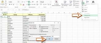
Select the percentage column. Right-click on it and select “Format Cells” from the context menu.

• In the format settings window, switch to the “Number” tab. Typically, this tab is open at the top of the window by default.
• Now pay attention to the field on the left side of the window that opens. It will be labeled “Number Formats”. Among the proposed options, you need to select “Interest”.
• Additionally, you can customize some aspects of how numbers are displayed, such as the number of decimal places.

Having displayed the result of one addition in this way, you can fill in the cells for the remaining products automatically. Select the cell in which you have already calculated everything and stretch it to the remaining products using a special manipulator in the lower right part. The data for the remaining cells will be inserted automatically according to the neighboring cells and columns that appeared in the formula.

Manipulating percentages in Excel is a fairly simple task. To execute them correctly, you just need to know a few formulas and correctly insert the necessary data into them.

How to subtract formulas in Excel. Simple calculations in Microsoft Excel. Addition and subtraction

Excel, using a tool such as formulas, allows you to perform various arithmetic operations between data in cells. Such actions also include subtraction. Let's take a closer look at how this calculation can be done in Excel.

Subtraction in Excel can be applied both to specific numbers and to the addresses of the cells in which the data is located. This action is performed thanks to special formulas. As in other arithmetic calculations in this program, before the subtraction formula you need to set = (=)

.
Then sequentially comes the minuend (in the form of a number or cell address), the minus sign (-)
, the first subtrahend (in the form of a number or address), and in some cases, subsequent subtrahends.

Subtract a number from a range of cells using the special Paste function

With this method you can do the following: Paste the number 99 into a blank cell and copy it. The specified number 99 is subtracted from the range of cells. Then delete the number.

Subtract a number from a range of cells with a formula

A simple formula can also help you here. Take the above data for example.

Batch subtracts a number from a range of cells without formula

And then all cells are extracted. And then the range of cells will be subtracted by the number. Note. If you want to create formulas, you can also check the "Create formulas" checkbox. If the selected cells include formulas and you do not want to subtract the calculated formula results, check the Ignore Cells Formula check box.

Let's look at specific examples of how this arithmetic operation is performed in Excel.

Method 1: Subtract numbers

The simplest example is subtracting numbers. In this case, all actions are performed between specific numbers, as in a regular calculator, and not between cells.

Recommended Productivity Tools

Try unlimited free for 30 days.
More details Download. Creating a budget is one of the easiest and most useful things you can do using a spreadsheet. When you use a spreadsheet, any changes you make to your budget are instantly updated across the entire budget, with totals calculated for you. You can use the same approach to create a household budget, a budget for a trip or a specific event, etc. Here's how to create a budget. It's surprising how often you find that you should have had another column or row, and while it's easy to insert them later, it's even easier to start with a small space. This makes it easy to insert a title or reorganize the design. . This is very different from how things work in most other programs, but you will find that it is a compatible spreadsheet feature.

After these actions are completed, the result is displayed in the selected cell. In our case, this is the number 781. If you used other data for the calculation, then, accordingly, your result will be different.

Method 2: Subtracting numbers from cells

But, as you know, Excel is, first of all, a program for working with tables. Therefore, operations with cells play a very important role in it. In particular, they can also be used for subtraction.

That's it for the income categories, so let's think about them. This illustrates how cells in your table can contain data numbers, text, images, etc. - or formulas. Let's continue creating a budget. Follow the same procedure to add the rest of the expenses.

To finish entering our budget information, we need to offset expenses and then figure out our net income by subtracting our total expenses from our total income. Figure. At this point, you have a working budget summary that should look like Figure.

Method 3: Subtract a cell from a cell

You can perform subtraction operations without numbers at all, manipulating only the addresses of cells with data. The principle of operation is the same.

We can fix this by adding a title and formatting the text and numbers. Allowing room for these headings is one of the reasons we left some space at the top and left when we first created the table. Let's make all the headlines bold. . Since we're dealing with dollar amounts, let's format the numbers as currency rather than just plain numbers. The Format Cells dialog box opens.

The situation looks much more readable now, but we can improve things a little further by highlighting the three most important values, total income, total expenses and net income. We could simply offset these numbers the same way we do in the headings, or you could choose any of several other options to highlight the values. Let's use some rows to offset these totals.

Method 4: Bulk processing of subtraction operation

Quite often when working with Excel, it happens that you need to perform a calculation of subtracting an entire column of cells by another column of cells. Of course, you can write a separate formula manually for each action, but this will take a significant amount of time. Fortunately, the application's functionality can largely automate such calculations, thanks to the autocomplete function.

One reason for this is that a workbook may contain multiple worksheets. Having descriptive names on your tabs not only makes it easier to quickly jump between worksheets, but it also helps if you end up developing more complex formulas that use values ​​from multiple sheets.

• This creates a boundary between the amount of income and the total amount of income.
• Repeat the process for the total cost.
• Top up your net income by applying multiple double boundaries.
• Let's rename this to more accurately reflect the contents of the worksheet.

Your table should now look like the image shown.
Using an example, we will calculate the profit of an enterprise in different areas, knowing the total revenue and cost of production. To do this, you need to subtract the cost from the revenue.

It's noticeably more readable, with important information. You can make him look a lot smarter if you want, but this is a good start. So the budget looks good, but is it delivering the right results? You can double check that the formulas you provided for total income, total expenses and net income are correct by making a small addition for yourself. You should also check if the formulas work by changing some of the amounts for income and expenses.

A simple spreadsheet makes it easy to check if your formulas are working. The steps in this tutorial assume that you have a cell containing the value you want to subtract. You can either subtract this value from the value in another cell, or subtract it from the number you select.

Method 5: Bulk Subtract Single Cell Data from a Range

But sometimes you need to do just the opposite, namely, so that the address does not change when copied, but remains constant, referring to a specific cell. How to do this?

If you want to subtract a cell value from a number that is not in the cell, replace one of your cells instead. The second value after the - operator. As with the first value, this can either be a different cell location or a numeric value.

• The = symbol is at the beginning of the formula.
• The first value after =.
• This can be either a cell or a numeric value.

For example, typing "=10-3" would show 7 in the cell even though there were no cell locations.
You can learn more about whether you're ready to start unlocking the potential of your current data. The above example is only a special case. In a similar way, you can do the opposite, so that the minuend remains constant, and the subtrahend is relative and changes.

As you can see, there is nothing complicated in mastering the subtraction procedure in Excel. It follows the same rules as other arithmetic calculations in this application. Knowledge of some interesting nuances will allow the user to correctly process large amounts of data using this mathematical action, which will significantly save his time.

Subtract by adding values ​​to the formula

If you need to display a formula instead of the result of a formula, then you will show what changes you need to make to do so.
However, the software does not have a subtraction function, which seems obvious. You don't need to enter any values ​​in the spreadsheet cells to subtract numbers. Instead, you can include the values ​​to subtract in the formula itself. First, select the cell to add the formula. For example, enter "=25-5" in the function bar and press Enter. The formula cell will return a value. The subtraction operation in the Microsoft Office Excel spreadsheet editor can be applied either to two specific numbers or to individual cells. In addition, it is possible to subtract the desired values ​​from all cells of a column, row, or other area of ​​the spreadsheet. This operation can be part of any formulas or itself include functions that calculate minuend and subtract values.

Subtracting references to spreadsheet tables

To subtract cell values, you will need to include their row and column references in the formula.

Subtract one number from each value within a range of cells

If you need to subtract one value from each number within a range of cells, you can copy the formula to other cells.

Subtract the value of a range of cells from a single value

What if you need to subtract the total number of columns for a group of cells from a single value?

Subtract two or more common values ​​from a range of cells

Instead, add cell range references to the formula and subtract them. Subtracting percentages from figures. To subtract a percentage value, such as 50%, from a number, you will need to enter the value in a cell with a percentage format. You can then add a formula that subtracts a percentage from a number in another cell.

You will need

• Microsoft Office Excel spreadsheet editor.

Instructions

• Click on the table cell in which you want to get the result. If you just want to find the difference between two numbers, first let the spreadsheet editor know that a formula will be placed in that cell. To do this, press the equal sign key. Then enter the number you want to reduce, add a minus number, and enter the number you want to subtrahend. The complete entry may look, for example, like this: =145-71. By pressing the Enter key, tell Excel that you are finished entering the formula, and the spreadsheet editor will display the difference of the entered numbers in the cell.
• If it is necessary, instead of specific values, to use the contents of some table cells as the subtracted, reduced, or both numbers, indicate links to them in the formula. For example: =A5-B17. Links can be entered from the keyboard, or you can click on the desired cell with the mouse pointer - Excel itself will determine its address and place it in the typed formula. And in this case, end your entry by pressing the Enter key.
• Sometimes you need to subtract a number from each cell in a column, row, or specific area of ​​a table. To do this, place the number you are subtracting in a separate cell and copy it. Then select the desired range in the table - a column, row, or even several unrelated groups of cells. Right-click on the selected area, go to the “Paste Special” section in the context menu and select the item also called “Paste Special”. Place o in the “Operation” section of the window that opens, and click OK - Excel will decrease the values ​​of all selected cells by the copied number.
• In some cases, it is more convenient to use functions instead of entering subtraction operations - for example, when the subtrahend or minuend must be calculated using some formula. Excel does not have a special function for subtraction, but it is possible to use its opposite - “SUM”. Call a form with its variables by selecting the line with its name in the “Math” drop-down list of the “Function Library” command group on the “Formulas” tab. In the Number1 field, enter the value to be reduced or a reference to the cell containing it. In the Number2 field, type -1*, and then enter the number to subtract, cell reference, or formula. If necessary, do the same with subsequent lines - they will be added to the form as you fill in the empty fields. Then click OK and Excel will do the rest.

Rate the article!
We recommend reading

Windows instructions
Kovalevsky on Russian national education

Smartphones
Japanese Economy in the Middle Ages

Android instructions
Taurus woman compatibility in love and relationships

Office programs
Luther opposed the idea that

Smartphones
See what “Treaty of Riga (1920)” is in other dictionaries Peace Treaty between Russia and Latvia

Windows instructions
Characteristics of the religious and philosophical trend in Russian psychology and the main periods of its development Who is the Russian philosopher Frank