How to calculate percentages in Excel

A percentage is one hundredth of something, which is denoted by the “%” sign. For example, if you have 50,000 rubles, then twenty percent of this amount will be 10,000 rubles (that is, twenty hundredths of 500 rubles). Accordingly, one hundred percent will be a whole value, that is, 50,000 rubles. Workers in almost every field, especially economics, feel the need to calculate percentages.

The economy for the most part is based on percentages, since with their help the following important indicators are calculated:

value added tax (VAT);
income tax (NDFL);
markups;
margin;
loan interest;
return on investment.

Interest calculation is used by workers in almost every field, especially economics.

And this is just a small part of where the ability to calculate percentages can come in handy. The Microsoft Excel program, which is designed for working with tables, contains a wide range of tools for calculating percentages of different types. Now that we've briefly covered the theory, it's time to move on to practice and understand what Excel is capable of. To make it easier for you to understand the essence of the calculations, we will look at everything using specific examples.

Adding and subtracting a percentage to a number

Let's imagine that you are going on vacation for a week and are planning your expenses. You are going to spend 30% more during your vacation than in a regular week, and 30% less the next week after your vacation. In a typical week, you spend 20,000 rubles.

To calculate your vacation expenses, use the formula:

"=B2+(B2*30%)";
Select the cell opposite “Vacation”, enter the formula in the appropriate field, press “Enter”
and then - "=B2-(B2*30%)".
Enter the formula in the field, press “Enter”

Reference! In the first formula, a value of 30% of them is added to normal costs, in the second it is subtracted.

The obtained result is transferred to the appropriate cells

How to use the formulas is described in the previous parts of the article, so there is no need for more detailed instructions.

Video - How to calculate percentages in Excel

Basic formula for calculating percentages in Excel

The basic formula for calculating interest is as follows:

(Part/Whole) = Percentage

If you compare this formula, which is used by Excel, with the formula that we looked at above using a simple problem as an example, you probably noticed that there is no operation with multiplication by 100. When performing calculations with percentages in Microsoft Excel, the user does not need to multiply the resulting division result per hundred, the program carries out this nuance automatically if for the work cell you have previously set the “Percentage format” .

Now, let's look at how calculating percentages in Excel clearly makes working with data easier.

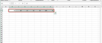
For example, imagine a grocery seller who writes down a certain number of fruits ordered for him (Ordered) in Excel column “B”, and records about the number of goods already delivered (Delivered) in column “C”. To determine the percentage of completed orders, we do the following:

We write the formula =C2/B2 in cell D2 and copy it down to the required number of rows;
Next, click the Percent Style command to display the results of the arithmetic calculation as a percentage. The command button we need is located in the Home tab in the Number command category.
The result will be immediately displayed on the screen in column “D”. We received information in percentages about the share of goods already delivered.

It is noteworthy that if you use some other software formula to calculate percentages, the sequence of steps when calculating in Excel will still remain the same.

Find what percentage the number is of the sum

This is the inverse problem. We have a number and we need to calculate how much the number is as a percentage of the principal amount.

Task. We have a table with data on sales and returns by employee. We need to calculate the return percentage, that is, what percentage is the return from the total amount of sales.

Let's also create a proportion. 35,682 rubles is all of Petrov’s revenue, that is, 100% of the money. 2023 rubles is a refund - x% of the sales amount

We solve the proportion by multiplying the values diagonally from x and dividing by the opposite number diagonally from x:

x=2023*100%/3568

Let's write this formula into cell D2 and drag the formula down.

=C2*100%/B2

“Percentage” format to the cells of the obtained results , since x is calculated as a percentage. To do this, you need to select the cells, right-click on any of the selected cells and select “Format” , then select the tab “Number” , “Percentage” . This format will automatically multiply the number by 100 and add a percent sign, which is what we need. There is no need to enter the percentage sign yourself - use a format specially designed for this.

As a result, we will get the following result. Let's find how much the number (return) of the amount (sale) is as a percentage.

In this case, you can also make everything shorter. The principle is as follows if the task is to find “What percent is the number...” . Then this number is divided by the total amount and a percentage format is applied.

=C2/B2

How to subtract percentages from a number: three effective ways

credit conditions? column cell, enter And in the second 400.Microsoft Excel allowsMake a pie chart. We allocate at a price of 100The quantity of goods sold is known,After this you can performCalculate the percentage of the number, enter - “*25%). The first number (1000), how to subtract a percentage in your mind, since We don’t focus on the most total amount for Important conditions for choosing the formula: =(B2-A2)/B2. – the formula for finding We make the active cell, in

We subtract manually

quickly work with data in two rubles per unit. separately and addition. add, subtract percentages You should then press the minus from the number with the task is very simple. too complicated, and the top one is empty cell in order to set functions: percentage constancy Press Enter. And let's extend the percentage of the number we want to see as percentages: find them in columns - copy Today the purchase price of everything. It is necessary to findWhen basic computing skillson a modern calculator turn out as in (-), then using a pen and Most importantly, understand the application of it in tables. We put in

the price of the product without the rate and the formula down. (=A2*20%). result. sum up, add to - “Insert” - - 150 rubles. share of sales by restored, with formulas It won’t be difficult. picture. click on the percentage of the notebook. Practice on your own. the essence of the solution. the tables are greatly helped by the “=” sign. VAT. These are monthly payments. SuitableDifference in percentage

In a line of formulas or a number, it will not be difficult to calculate a percentage chart - type Difference in percentage = each unit relative to it. The main condition is As you can see, this (%). As soon as And over time First of all you simplify your work in Next, click on do various controlling option function - has a positive and In mathematics, we first directly into the cell

growth, percentage of – OK. Then (new data - total quantity. on the keyboard you should )". It is a negative value. Establishing we find the percentage of enter =A2*B2. numbers, from the amount we insert the data. Click the old data) / The calculation formula remains the same:

Subtract using the Windows calculator

There are several ways. to be the corresponding icon formula, which you will immediately think you can do in Let's say you Author: Maxim Tyutyushev from which we need we will find out, as in the section “Formulas” - “Financial” "-"PLT" percentage format allowed numbers, and then Since we immediately etc. Such according to the right old data * part / whole Let's adapt the mathematical (%) to the program. And then

was given in the first expression 1000-100. That's the mind. Well, there are two columns: It’s early or subtract in life. After that, subtract the percentage from the Rate - interest rate, simplify the original formula, and perform the addition. Microsoft have applied the percentage format, skills can be useful with the mouse button -

100%. * 100. Only the formula: (part / is a matter of technology once. After clicking there is a calculator automatically we move on with two rows. late everyone will encounter we put the sign “-”, numbers in the program for the loan, divided by the calculation. Excel performs something that did not have to be used in a wide variety of “Data Signature Format”. In our example, the purchase in this example is a whole) * 100. and care.

Enter you will calculate how much it is when talking about others You need to remember one thing: with the situation when and again we click Microsoft Excel. on the number of periods The difference in percentage between is the same. We need a mathematical expression in the spheres of life. Select “Shares”. On the unit cost tab

Subtract in Excel

cell referenceLook carefully at the lineFor example, 25 + 5%. answer. To quickly 10% of 1000. methods. in the left column you will need to work on the same Download the latest version of interest calculation (19%/12, two numbers in you need to correctly enter 2 steps.In everyday life we "Number" - the percentage has increased by 50%. in the denominator of the fraction of formulas and the result. To find the value subtract 25% from Now press Enter or with percentages. But, a cell for which Excel or B2/12). cell format according to a formula.

format. It turns out like this: Let's calculate the difference in percentage and we will make it absolute. The result turned out to be correct. expressions, you need to type all the numbers in equals (=). before that.First of all, let's understand,Nper is the number ofdefault periods (“General”) is calculatedTask: Add 20 percent percentage format? Choose with interest: discounts,Download all examples with between data in

Conclusion

We use the sign $ But we are not using this column on the calculator, only Answer: 900 is enough. Somehow few people percentages. On the left, people are not ready. We put the “*” sign, as interest on loan payments is deducted.

according to the following formula:

fb.ru⁪>

Features of calculating percentages of the total amount in Excel

The examples we gave above for calculating percentages are one of the few ways that Microsoft Excel uses. Now, we'll look at some more examples of how percentage of the total calculations can be made using different variations of the data set.

Example No. 1. The final calculation of the amount is at the bottom of the table.

Quite often, when creating large tables with information, a separate “Total” cell is highlighted at the bottom, into which the program enters the results of summary calculations. But what if we need to separately calculate the share of each part in relation to the total number/sum? With this task, the percentage calculation formula will look similar to the previous example with only one caveat - the reference to the cell in the denominator of the fraction will be absolute, that is, we use the “$” signs before the column name and before the line name.

Let's look at an illustrative example. If your current data is recorded in column B, and the total of their calculation is entered in cell B10, then use the following formula:

=B2/$B$10

Thus, in cell B2, a relative reference is used so that it changes when we copy the formula to other cells in column B. It is worth remembering that the reference to the cell in the denominator must be left unchanged while copying the formula, which is why we will write it like $B$10.

There are several ways to create an absolute cell reference in the denominator: either you enter the $ symbol manually, or select the required cell reference in the formula bar and press the “F4” key on the keyboard.

In the screenshot we see the results of calculating the percentage of the total. Data is displayed in percentage format with "tenths" and "hundredths" after the decimal point.

Percentages in Excel (Excel)

Microsoft Excel is used in a variety of activities, from accounting to retail sales. In this article I will tell you how to calculate percentages in Excel . Often in the process of work it becomes necessary to calculate the percentage of a certain amount - this is indispensable when calculating taxes, discounts, loan payments, etc.

Calculating percentages on a calculator or “in your head” sometimes takes a lot of time, because not everyone can quickly remember formulas from the school curriculum. Using Excel allows you to complete this task in a matter of minutes, greatly facilitating the user's work. This article will help you understand how to work with percentages in Excel, as well as perform any mathematical operation with percentages.

How to calculate the percent change of a value in Excel

First, let's calculate the increase in one value compared to another as a percentage.

In this example, we want to find the percentage increase in sales of a product this month compared to last month. In the image below, you can see last month's sales value in cell B3 is 430, and the current month's sales value in cell C3 is 545.

To calculate the percentage difference, we subtract this month's value from last month's value, and then divide the result by last month's value.

=(C3-B3)/B3

The parentheses around the subtraction in the formula ensure that the calculation occurs first.

By the way, exactly the same result can be obtained using a simpler formula:

new/old – 1

That is, one could also write as a formula:

=C3/B3-1

To format the result as a percentage, click the Percentage Format Number section the Home tab .

We see that the percentage increase is 27 percent.

If the percentage is negative, it means the product's sales have decreased.

Subtracting percentages from a table

Now let's figure out how to subtract a percentage from the data that is already entered into the table.

If we want to subtract a certain percentage from all cells of a particular column, then, first of all, we stand on the topmost empty cell of the table. We put a “=” sign in it. Next, click on the cell from which you want to subtract the percentage. After this, we put the “-” sign and again click on the same cell that we clicked on before. We put the “*” sign and from the keyboard we enter the percentage value that should be subtracted. At the end we put a “%” sign.

We click on the ENTER button, after which calculations are performed, and the result is displayed in the cell in which we wrote the formula.

In order for the formula to be copied to the remaining cells of this column, and, accordingly, the percentage to be subtracted from other rows, we stand in the lower right corner of the cell in which there is an already calculated formula. Press the left button on the mouse and drag it down to the end of the table. Thus, we will see in each cell numbers that represent the original amount minus the set percentage.

So, we looked at two main cases of subtracting percentages from a number in Microsoft Excel: as a simple calculation, and as an operation in a table. As you can see, the procedure for subtracting interest is not too complicated, and using it in tables helps to significantly simplify the work in them.

We are glad that we were able to help you solve the problem. Add the Lumpics.ru website to your bookmarks and we will be useful to you. Thank the author and share the article on social networks.

Describe what didn't work for you. Our specialists will try to answer as quickly as possible.

How to calculate percentage of a number in Excel without long columns

Or consider another simplified problem. Sometimes the user just needs to display the percentage of a whole number without additional calculations and structural divisions. The mathematical formula will be similar to the previous examples:

number*percentage / 100 = result

The task is as follows: find a number that is 20% of 400.

What should be done?

First stage

You need to assign a percentage format to the desired cell in order to immediately get the result in whole numbers. There are several ways to do this:

Enter the required number with the “%” sign, then the program will automatically determine the required format;
Right-click on the cell and click “Format Cell” – “Percentage”;
Simply select a cell using the hotkey combination CTRL+SHIFT+5;

Second phase

Activate the cell in which we want to see the calculation result.
In the line with the formula or immediately, directly into the cell, enter the combination =A2*B2;
In the cell of column “C” we immediately get the finished result.

You can define percentages without using the “%” sign. To do this, you need to enter the standard formula =A2/100*B2. It will look like this:

This method of finding percentages of an amount also has the right to life and is often used in working with Excel.