Methods
Each of us can understand something different by rounding, so let's look at what options are available in Excel:
- Simple discarding of the fractional part. For example, we have the number 12.3456, but we want to see only tenths and hundredths; we are not interested in greater accuracy. By discarding the fractional part we get the result 12.34. This method is often used for beauty, so as not to overload the table and yourself with unnecessary signs. In this case, you can use the cell format to solve the problem.
- Mathematical rounding. In this case, some of the decimal places are discarded, but the next digit after the digit that is significant for us is taken into account. We look to see if it is more than 5 or less. For example, we have the number 12.57. We want to round it to the nearest tenth. Then, according to the rules of mathematics, we get 12.6. That is, we increased the tenths by 1, because hundredths are greater than 5. If we rounded 12.52, we would get 12.5.
- Rounding to the nearest higher or lower number is called rounding up and rounding down, respectively. For example, we have the original data: 12.75, 12.31, 11.89, which we want to convert to integer values. If we round down, we get 12, 12, 11. If we round up, we get 13, 13, 12.
- Rounding to tens, hundreds, thousands, and so on. This option is useful when we need approximate calculations, without detail.
- Round to the nearest even and odd value.
- Rounding to the nearest multiple of a number. For example, we have 124 candies, and 1 box holds 13 candies. And we want to understand how many candies we can fit in boxes of 13 pieces. Then we will round 124 to the nearest integer multiple of 13 and get the result 117.
For each of these cases, Excel has its own rounding function. Let's learn how to use them. But first, let's see how you can change the appearance of the data in the table.
Rounding numbers to digits in Excel
Excel has a standard function ROUND , which allows you to round a number by the number of digits:
ROUND(number, number_places) Rounds a number to the specified number of decimal places.
- Number (required argument) - the number to be rounded;
- Number of digits (required argument)—number of digits for rounding.
Example of using the ROUND formula
Cell Format
Often we don't want actual rounding, but just a neat, uniform look for all the numbers in the table. In this case, we do not use formulas, but simply change the appearance of the data.
To do this, select the cells in the table and press the right mouse button. In the context menu, select the desired section.
In the “Number” tab, select the appropriate format.
“General” is used by default and displays the data in the cells as they are; you cannot change the appearance here.
“Numerical” allows you to display as many decimal places as needed, or remove the fractional part altogether.
“Currency” and “Financial” are similar to “Numeric”, but also allow you to specify a currency.
In “Percentage” you can also adjust the number of decimal places. If we switch to this format, the original data in the cells is multiplied by 100 and a % sign is added.
I most often use the number format for my calculations. It is universal and allows you to quickly bring cells to a single look.
This method is suitable for Excel of any year. If you have a new version of the program, you can solve the problem even faster. For this purpose, there is a special block of options in the “Home” tab. Here you can select the appropriate format from the drop-down list, and use the left and right arrows to increase or decrease the number of digits.
Please note: changing the data format does not change the actual values in the cells, they remain the same, they are just displayed differently.
How to work with functions in Excel
We looked at the easiest way to remove unnecessary signs. It is quite convenient to use if we do not need to change the data in the table itself. Now we move on to using the various functions. But first I want to remind you what they are and also how to work with them.
Functions make calculations faster and easier. For example, we need to calculate the sum in a column that has 100 values. We can do this in the most direct way “1+20+30+43...” and so on 99 times. Or write the built-in “SUM” command, specify a range of cells, and the program will do the calculations in a second.
First way
To manually write a formula in a cell using a function, you must:
- Put the = sign.
- Specify the name correctly.
- Open parenthesis.
- Specify the arguments separated by semicolons, that is, the data that will be used.
- Close the bracket.
What can serve as an argument for mathematical formulas:
- number,
- formula,
- range of cells.
Example: the function “=SUM(F21:F30)” will calculate the sum of the numbers written in column F from position F21 to F30.
These rules must be remembered, otherwise the program will not be able to make calculations, but will produce an error of this type.
Second way
If it is inconvenient to write commands manually, then you can use the library, which is located in the “Formulas” tab.
We are currently interested in mathematical operations. Click on the appropriate section and select the desired procedure.
This will open a dialog box that makes it easy to understand what arguments you need to provide. Fill in the fields and click “OK”.
Dropping the fractional part
This method is suitable if we do not care whether rounding occurs according to mathematical laws and in which direction the value will change. When we simply want to simplify calculations by removing unnecessary signs, we can discard them. To do this, there is a function “SELECT”, which contains 2 parameters:
- the number on which the action needs to be performed;
- number of decimal places to leave.
For example, we have a product price of 4,716 rubles 77 kopecks and a lot of decimal places. It is logical to discard everything unnecessary and get only rubles and kopecks.
If we want to receive only rubles without kopecks, then as the second argument we write not 2, but 0.
Mathematical rounding
For the mathematical operation familiar to us from school, there is a special function “ROUND”. It is needed to work with fractional parts and integer values. The arguments are the number and number of digits to be left after the decimal point.
For example, we have a value of 34.83021 and we want to round it to the nearest hundredth. Then the formula will look like this: “=ROUND(34.83021;2)”.
If we specify 0 as the second argument, we will get an integer value, that is, we will round the initial data to units. And if the number of digits is negative, then an integer will be converted.
For example, we want to round to the nearest hundred 1245.329. Then we make the following entry in the cell of our table: “=ROUND(1245,329,-2)” and get the result 1,200.
Examples of using rounding functions
=ROUND(1.475,2) Rounds the number 1.475 to two decimal places, resulting in 1.48;
=ROUNDUP(3.14159,3) Rounds 3.14159 to three decimal places, resulting in 3.142;
=ROUNDDOWN(3.14159) Rounds down 3.14159 to three decimal places, resulting in 3.141;
=ROUND(10,3) Rounds the number 10 to the nearest multiple of 3, which is 9;
=ROUNDUP(2.5,1) Rounds the number 2.5 to the nearest higher multiple of 1, which is 3;
=OVERDOWN(2.5,1) Rounds the number 2.5 to the nearest smaller multiple of 1, that is, to 2.
In order to avoid possible inaccuracies and errors, you should carefully select formats and rounding methods when creating tables in Excel. If the tables are not already formed exactly as you would like, then the tabular data can be processed programmatically using VBA using macros.
Down and up
It happens that we do not need an exact mathematical calculation, but it is important not to exaggerate or, conversely, not to decrease the value in a cell. Then we will round down or up.
Up to fractional parts
To round down or up, there are universal functions “ROUND DOWN” and “ROUND UP”. They allow you to make conversions accurate to integer and fractional parts.
The first argument is the number to be rounded. The second is the number of digits. If it is greater than 0, then it shows how many decimal places should remain; if it is less than 0, then rounding occurs to tens, hundreds, thousands. If the argument is 0, then we get precision to units, the fractional part is discarded.
Let's look at an example of how these two commands work.
Up to whole
There is another way to round down or up. To do this, we need the “OKR-DOWN” and “OKR-UP” functions. They are used to obtain an integer result.
The second argument shows to what digit we are rounding:
- 10 – up to tens;
- 100 – up to hundreds;
- 1,000 – up to thousands, etc.
I show with an example.
Rounding down to units can be replaced by the “INTEGER” function, which has a single argument – a number. The result will be the same as when using “OKRVNIZ”.
The “EVEN” and “ODD” actions help to round up to the nearest even or odd integer value. You can see an example of using one of them in the screenshot.
Up to integers, taking into account multiplicity
Remember the example with candy that was at the beginning of the article? Now we will learn how to round to the nearest multiple of a value. For this purpose, there are 2 functions: “OKRV.MAT” and “OKRV.MAT”. The first reduces the original value, and the second increases accordingly.
For example, let's say we have the number 124 and we want to round it to the nearest higher multiple of 5. Then we write in the cell: “=OVERTOP.MAT(124,5)” and as a result we get 125.
How to round numbers up and down using Excel functions
one sign is left with the right mouse button, assignments and properties. database, the amount Formula "ROUND" the number of sheets set INTEGER - rounds to The following example demonstrates automatically adjusted. If =ROUND(A1;5) which will return the value 0=ROUND(number,precision) q. Let's use the following
rubles, then from and returns the rounded down. the “ROUND DOWN” function is applied. after the decimal point, 2 call the menu “Format Thus, this program values. These functionsThe result of any calculation, so by the user. of a whole. this feature: it will be necessary to replace such A1 - (0,3 Description of arguments: formula: the first value will be subtracted. For example, for Round to an integer in Example formula: =ROUNDBOTTOM(A1;1). – two and cells." Doing this is an indispensable assistant similar to the sum function
How to round a number using cell format
the same as Each sheet of the program represents RUN - discards the fractionalROUND(number; number_digits) results old prices this is a universal designationBoth arguments number andnumber are a required argument,=B2*B3*B4/1000 unit, otherwise the number will be rounded to 1.22365
Excel can be used with Result: etc.).
the same thing is possible
for any people in Excel type sum in Excel,
is a table consisting of
returned simply rounded to two digits using the “ROUND UP” functions Formulas “ROUND UP” and “ROUND DOWN” Now let’s round the integer
via the “Number” tool
How to properly round a number in Excel
professions that are so "SUM". may be subject to rounding. from 65536 lines EVEN and ODD -As arguments to the function in a personal message, I will explain andAlik the Striped Giraffe
taken from the range
- function ROUND; use the formula: value.
- After the comma you can also use “OKRVNIZ”. Rounding are used for rounding (not a decimal). on the main page or otherwise related "CELL" Rounding in Excel and 256 columns. round to the next ROUND can protrude
this.: Damn, this is the impression, only positive or
- accuracy is a required argument,0;B5-INTEGER(B5)0.5;B5-INTEGER(B5)
- Calculation result: enter the formula =ROUND(1.22365;2), occurs in large values of expressions (products, Use the function ROUND: Books. Or press with numbers and - this function
How to round a number to thousands in Excel?
It is important not to confuse Every cell is like this
whole: even or
numbers, text representations Beth Midler what are you, madam
only negative numbers characterizing a numerical value In this case, the function That is, 2200 rubles which will return the value or the smaller side
sums, differences andthe first argument of the function - hotkey combination
How to round up and down in Excel
numbers. provides the user with information displaying the value.
table is called a cell. of odd. numbers, links to: stand on the cell.
Not even once respectively. If the number is the accuracy of rounding the number. IF it performs a check you can change not 1.22. to the nearest integer
etc.).
cell reference;
CTRL+1.Author: Anastasia Belimova about the properties of a cell.
To perform an action
An Excel cell has its own
The following example shows cells with numeric in the menu click did not open the table is positive, but
How to round to a whole number in Excel?
Notes: the fractional part found more than the ROUND function is used for the number. To round the second argument to a whole number - with Select a number format and Round numbers in Excel Mathematical functions “rounding in Excel” individual address consisting of the action of the ROUND function
data, as well as the “format” command, select in Excel. How accuracy - negative Functions ROUND and ROUND power values by 31 cu rounding numbers with Example of using functions: upwards
sign "-" (before
We set the number of decimals in several ways. C is the core of Excel. You need to select a cell from the row number with negative, positive formulas and functions.
"cells". then ask you to explain... or vice versa, the function is taken as belonging to the interval required accuracy andThe second argument is an indication
use the “ROUND UP” function. tens – “-1”, signs – 0.
using the cell format Calculations with their containing the result of the calculation, and a Latin letter and equal to zero Both arguments are required. the value of “numeric” and A1 is
ROUNGLT will return the code
arguments are numeric values of values from 0 Example 2. A car's speedometer returns a rounded value. by digit, to To round to to hundreds -
Rounding result: and using using - put the main in front of the number
column (for example, 1A,
Why does Excel round large numbers?
the second argument. The number in the box is the cell address. Error addresses #NUMBER and text representations up to 0.25 and displays the speed in the ROUND function accepts which integer must occur to the lesser "-2" to round Assign the number of decimal places to functions. These two are the purpose of the program. In the equals sign (“=”), 2B, 5C).In this example, in(number) is the value, decimal places in Excel consist of Rounding direction (upward or numbers. ROUND function
exceltable.com>
In Google Sheets
If you like to work online, you can set up a rounding formula in Google Sheets.
To change the cell format, use the option on the main toolbar.
There is also a corresponding tool to reduce or increase the bit depth.
To open a list of built-in formulas, click on the small black triangle next to the sum icon.
To round data in cells, hover over the mathematical functions and select one of the options:
- OTBR,
- ROUND,
- ROUNDUP,
- ROUND BOTTOM
- OKRVVERH,
- OKRVNIZ,
- WHOLE,
- EVEN,
- ODD
They work in exactly the same way as in Excel, but in Google Sheets there are no “CORN BOTTOM.MAT” and “COVER UP.MAT” actions. Instead, you can use “ROUND”, this function rounds to the nearest multiple of a certain number. That is, in this case, the program itself decides whether the original data will change more or less.
Round up or down
Excel provides other tools that allow you to work with decimals. One of them - ROUND UP , gives the closest number, the largest in modulus. For example, the expression =ROUNDUP(-10,2,0) will give -11. The number of digits here is 0, which means we get an integer value. The nearest integer , larger in modulus, is just -11. Usage example:
Ways to create a table in Microsoft Excel
ROUND BOTTOM is similar to the previous function, but returns the closest value with a smaller absolute value. The difference in the operation of the above tools can be seen from the examples :
| =ROUND(7.384,0) | 7 |
| =ROUNDUP(7.384,0) | 8 |
| =ROUNDBOTTOM(7.384,0) | 7 |
| =ROUND(7.384,1) | 7,4 |
| =ROUNDUP(7.384,1) | 7,4 |
| =ROUNDBOTTOM(7.384,1) | 7,3 |