How to search for values in Excel.
Search in Excel
The following describes several options for searching and filtering data in an Excel table.
Classic search "MS Office".
Conditional formatting (highlighting the desired cells with color)
Setting up filters based on one or more values.
A fragment of a macro for iterating through cells in a range and finding the desired value.
Finding the right data in a range
15124 28.10.2012
How to use the VLOOKUP
To search and select the required values from the list, we recently analyzed. If you are not yet familiar with it, take a look here, don’t regret five minutes to save yourself several hours later.
If you are familiar with VLOOKUP, then - to catch up - it is worth understanding similar functions: INDEX
and
MATCH
, the knowledge of which will greatly facilitate the life of any experienced Excel user. Take a look at the following example:
It is necessary to determine the delivery region by the product article typed in cell C16.
The problem is solved using two functions:
=INDEX(A1:G13,MATCH(C16,D1:D13,0),2)
MATCH function
looks in column
D1:D13
for the value of the article from cell
C16
. The last function argument 0 means searching for an exact (not approximate) match. The function returns the serial number of the found value in the range, i.e. actually the line number where the required article is found.
INDEX function
selects from the range
A1:G13
a value located at the intersection of a given row (the line number with the article is given by
the SEARCH
) and column (we need the region, i.e. the second column).
Related links
- Using the VLOOKUP function to search and substitute values.
- Improved version of the VLOOKUP function
- Reusable VLOOKUP
Pages:
Andrey
28.10.2012 23:19:31
and how to solve the problem? For example, I have a table and I need to find a number using 2 parameters (for example, using x and y values). Link
Elena
28.10.2012 23:19:52
Andrey, your problem is solved in a similar way, only after searching for the row number (x), the column number (y) is searched in the same way. =index(data_array,(search(row_number,row_array,0));(searchpos(column_code,column_array,0))). Parent Link
Hovik Ghambaryan
25.11.2014 13:30:23
Hello, I also have a problem on this topic, the thing is that you need to search in a small database for two matches, Moscow is in one cell and 002 is nearby and there is a sheet in which there is also Moscow and 002 is nearby, it’s just that there are a lot of 002 and Moscow, but I want, first of all, the formula found exactly the Moscow with which 002 eats next and the second in the first sheet next to Moscow and 002 is written 10, and on the second sheet next to Moscow 002 eats 5 I need the formula to find these numbers and multiply them, please help me This already gives me a headache but nothing works Parent Link
kep
28.10.2012 23:20:30
Oops, everything is fine when the desired value is found, BUT, if the desired value is not found, then the function returns “#N/A” QUESTION: how can I make the cell value equal to zero instead of “#N/A”? Link
Nikolay Pavlov
28.10.2012 23:26:41
Use, for example, the IFERROR function - it intercepts any errors and displays any value you need (0) instead. Parent Link
Galina
28.10.2012 23:21:40
Many thanks to those who made this site, with the help of it I solved my problem. Link
Nikolay Pavlov
28.10.2012 23:26:55
My pleasure! Parent Link
Leonid
28.10.2012 23:22:36
Very useful site! A huge plus is that the names of the functions are given in both Russian and English - a good way to access the site from search engines. The combination INDEX+MATCH can be used if you need not only to select one value from the original table, but also entire rows (for example, from a sales table in which subtotals by month are also calculated, transfer only rows with subtotals to a new table). Solution: in the INDEX and MATCH functions, freeze the ranges completely in each, and also freeze the cell for which a match is being searched so that it does not shift along the columns. Example:
| =INDEX($A$311:$J$778,MATCH($A790,$C$311:$C$778,0),2) |
Link
Parviz
28.10.2012 23:24:09
Hello, I have a question about this example: =INDEX(A1:G13,MATCH(C16,D1:D13,0),2) what is the number 2? Link
Nikolay Pavlov
28.10.2012 23:27:41
this is the column number in the table from which we take the value, i.e. region Parent Link
Dmitriy
28.10.2012 23:25:36
Additional condition to the problem: Let’s assume that product article 8985 has not one, but two regions. Is a solution possible if the regions are written in one cell? Link
Nikolay Pavlov
28.10.2012 23:28:52
You can extract all occurrences, not just the first one, using an array formula - see here Parent Link
Alexander R
01.01.2013 01:43:20
Please tell me what if article 6576 is repeated twice in the range D1:D13, but the delivery regions for it are different. How best to solve the current problem of “determining the delivery region by the product article typed in cell C16”
? Link
Nikolay Pavlov
03.01.2013 00:02:23
The above formulas will give you the first region encountered. If you need to display all regions for a given article, you will have to use more tricky constructions - see Reusable VLOOKUP Parent Link
Alexander R
04.01.2013 02:08:28
Thank you for your reply. To be honest, I was faced with a slightly different task. But it was with the help of this topic and information from your forum that we managed to solve it. Thanks again. Parent Link
Tatyana Danilova
27.11.2019 13:39:27
The chance of getting an answer is negligible, but suddenly... I also need to display the sum of all values when entering several conditions, and SUMIFS is not suitable, because the values to be summed are not just in one column. What formula did you manage to create? Parent Link
Joric
09.01.2013 14:48:34
Tell me, please, is it possible for this wonderful formula to look for values on different sheets? I tried to do this: =IFERROR(INDEX(Sheet2!C700:F900,$C$700:$F$900,MATCH($A700,$C$700:$C$900,0),1),0), but nothing it turns out... Thank you. Link
Nikolay Pavlov
11.01.2013 18:06:51
It's hard to say without a file. But right off the bat, what is highlighted in red in your formula? =IFERROR(INDEX(Sheet2!C700:F900,$C$700:$F$900,MATCH($A700,$C$700:$C$900,0),1);0) The INDEX function has three arguments, and you have - four. Something extra Parent Link
atas
11.04.2013 08:07:19
Of course you can. I had a similar task and it only worked with INDIRECT. In my case, the names of the sheets are in column A. (I just couldn’t figure it out with a large number of quotes, but it works) =INDEX(INDIRECT("'"&$A5&"'!$A$8:$Z$50");MATCH($ M$1;INDIRECT("'"&$A5&"'!$B$8:$B$50");0);J$4) Parent Link
Elena
13.01.2013 10:11:19
Good afternoon. When I change the value by which I need to search, the found values do not change automatically, only if I click on this cell and Enter, or by saving the file. What can be done? Link
Nikolay Pavlov
13.01.2013 11:53:44
Apparently you have turned off automatic recalculation of formulas. Tab - Calculations - Automatic
. Parent Link
Irina
08.02.2013 08:36:20
Hello, Nikolay. I would like to ask you to help me with the solution: on one page there is a range of cells in 4 columns, you need to set a condition that if in the range of cells of the fourth column there is 0, then you need to select a value from the second left column and put it in a certain range of cells on another sheet, and already the value is 100 (that is, in the 1st sheet O, then on the 2nd sheet 100 and the sum of all these “100”;). Question: which function to choose. And the second question: On the Internet, I open my Qiwi wallet and see the amount, but is it possible to use a hyperlink so that the program can see the balance of the wallet at the moment without going to the Internet? Thank you in advance. Irina Link
Nikolay Pavlov
08.02.2013 09:57:17
Irina, with questions not on the topic of the example, it’s better to go to the forum. Create a topic, attach a file, describe the situation and the desired result. Here are the comments for example. And it’s impossible to answer your question without seeing your file - even if you want to. Parent Link
Lisa
11.02.2013 08:40:14
When using MATCH, I encountered a problem: I need to find a cell not by its exact value, but take the nearest smaller value and the nearest larger value. Finding a smaller value without any problems. When searching for more, it returns #N/A. Maybe you know why this is so? Link
Nikolay Pavlov
11.02.2013 10:38:40
When searching for the nearest smallest (the last argument of the MATCH function is 1), the table where we are looking must be sorted in ascending order. When searching for the nearest largest - in descending order. Is it like this for you? Parent Link
Lisa
11.02.2013 11:02:24
Now it is. Thank you. Parent Link
Yuri
05.04.2013 19:55:31
Please tell me if instead of the product article (in the example) it is necessary to substitute text. I tried it and it says #N/A. I tried to set the range (of articles) as text, but it still gives an error. What should I do to fix it? Link
Nikolay Pavlov
11.04.2013 08:05:42
If you mean to substitute the name of the range with text instead of the usual range selected by the mouse, then you will have to use the INDIRECT function, which will turn the text name of the range into a real link to it. Parent Link
INFINITY
12.05.2013 06:40:07
Thank you very much, Nikolay! Not only for this example, but in general - for the entire Site!!! Link
Anton Popov
20.05.2013 19:14:12
Nikolay, thanks for the lesson! Wouldn't it be better to do the same using the VIEW function? =VIEW(C16;D2:D13;B2:B13) I think it’s easier to understand and implement. Link
Nikolay Pavlov
26.05.2013 09:50:32
Thanks for the clarification, Anton! VIEWING is also an option in some cases. Parent Link
Arthur Manukyan
26.05.2013 14:47:05
Good day to all! This is my first comment. First of all, I would like to thank Nikolai for his work and for this site. Everything is very clear, structured and very useful in everyday work. This resource is in first place in my Excel tabs! Well, now on the question, if I may, regarding the index function, which is used in this example. Please tell me what to do if the table is in another adjacent sheet. The method indicated above works exactly up to the 3rd field of the index function, where we need to indicate the desired column in the form of a number, from where we take the value (client name, region, etc.) How to correctly perform this stage in order to take these values from the adjacent sheet ? Thank you in advance for your help! Link
Nikolay Pavlov
30.05.2013 13:11:27
Specifying the sheet name and cell address, where to get the column number from, like Sheet1!A1 - doesn’t help? Parent Link
Andrey
31.08.2014 00:07:53
Doesn't always help. Today I spent the whole day implementing this method. I can’t understand everything - either the office on the computer is crooked... or one of the two... then #returns the link or #n/a. =INDEX(Dealers!$A$4:$B$103;C3;2) on one sheet it worked after the millionth attempt on another sheet it doesn’t work at all. Why it worked on the first one is unclear. It just gave the desired result at some point and that’s it. Although I didn’t touch anything in the formula. If you insert MATCH it doesn’t work at all. I liked the potential of the function, but I didn’t like how it worked for me specifically. VLOOKUP works perfectly, but only on one sheet. On the other hand, he doesn’t even want to break up. I really liked your resource. I picked it up. Thank you. Parent Link
Andrey
17.09.2014 12:51:13
Hm. I finally overcame it. great feature! made my job so much easier!!! THANK YOU SO MUCH NIKOLAY!!! Parent Link
elena farafontova
30.05.2013 11:44:06
Greetings! How to search a range using two positions at the same time? Those. if, in the example in the Data Search topic, the region and the desired price (approximately) are known in the range, but you need to find and display the quantity in a cell. INDEX AND MATCH have the same meaning. Thank you in advance) Link
Nikolay Pavlov
30.05.2013 13:07:05
If you are looking exactly, you can simply pre-combine two columns into one using the CONCATENATE function to get one column to test the conditions. If you need to look approximately, then there is no simple solution. Parent Link
elena farafontova
02.06.2013 13:54:36
Thanks to Nikolai for the incredible combination of VLOOKUP functions; OFFSET; MATCH; COUNTED, which gave me a lot of free time. Very competent.8) Link
Vasily Eriklintsev
07.08.2013 10:28:25
Nikolay, good afternoon! Excellent formula I use it very often, however I encountered a small problem, I pull the substituted data from another file, i.e. In the formula I have a link to another file. And very often when you open a file with the formula INDEX (SEARCH...) it is covered with links, the only cure is opening the file to which there is a link in the formula. It’s not critical, of course, but sometimes it’s very inconvenient. Is there any way to cure this? Link
Lyudmila Gobova
09.08.2013 13:42:49
Hello, Nikolay! I have this task. The document contains three pages of information (3 classes: A, B, C), each of which has a different number of students. On page 4, in the protocol, I need to display information separately about each of the students who studies in one of the three classes. How to get information using the “index” function by student number and class. Those. I’m interested in the second option for using the “index” function, how to search in several tables, how to write the formula correctly. Sincerely, Ludmila. Link
acheslav
18.09.2013 21:48:36
Nikolay, thank you very much for your lessons! After watching this lesson and downloading your example, I found a solution to my problems. In particular, instead of specifying the column number, I inserted MATCH =INDEX(A1:G13,MATCH(C16,D1:D13,0),2) =INDEX(A1:G13,MATCH(C16,D1:D13,0);MATCH(B17; A1:G1;0)) Thank you again! Best regards, Vyacheslav! Link
Nikolay Pavlov
21.12.2013 09:54:48
Well yes, a good solution to not count the column number manually Parent Link
Anton Zolotukhin
11.08.2014 09:44:33
Hello, is there a solution if the table header is multi-layered? Multi-layer header - for example, in row 2 conditions in column there are 2 conditions and not one at a time. those. =INDEX(Table value range; MATCH(column A header value, column A header range, 0); MATCH(row 1 header value, column header range 1,0); and I need to add 2 more conditions MATCH(column B header value ;column header range B;0); SEARCH(row header value 2;column header range 2;0); i.e. the ready value will be selected not by 2 conditions, but by four. Please tell me how to implement this in one formula. Thank you !Parent Link
Nikolay Pavlov
11.08.2014 10:01:17
Anton, how can I answer you without seeing your file? It’s better to create a topic on the forum, attach a file - we’ll help. Parent Link
Anton Zolotukhin
11.08.2014 10:36:48
You answered so quickly that I didn’t have time to draw the table)) =INDEX(Range of table values; MATCH(value of column header A; range of column A header; 0); MATCH(value of row header 1; range of column header 1; 0);
| Condition 2 | q | q | q | h | h | h | |||
| Condition 4 | x | y | z | x | y | z | |||
| condition selection list 1 | k | Condition 1 | Condition 3 | ||||||
| condition selection list 2 | q | j | b | A | b | V | G | d | e |
| condition selection list 3 | j | s | e | and | h | And | To | l | |
| condition selection list 4 | j | f | m | n | O | P | R | With | |
| solution | T | k | b | T | at | f | X | ts | h |
| k | s | w | sch | ъ | s | b | uh | ||
| k | f | Yu | I | — | — | — | — |
and I need 2 more conditions to add SEARCH(the value of the header of column B; the range of the header of column B; 0); MATCH(row header value 2;column header range 2;0); those. the finished value will be selected not according to 2 conditions, but according to four
| Condition 2 | q | q | q | h | h | h | |||
| Condition 4 | x | y | z | x | y | z | |||
| condition selection list 1 | k | Condition 1 | Condition 3 | ||||||
| condition selection list 2 | h | j | b | A | b | V | G | d | e |
| condition selection list 3 | s | j | s | e | and | h | And | To | l |
| condition selection list 4 | j | f | m | n | O | P | R | With | |
| solution | #LINK! | k | b | T | at | f | X | ts | h |
| must be s | k | s | w | sch | ъ | s | b | uh | |
| k | f | Yu | I | — | — | — | — |
Parent Link
Nikolay Pavlov
11.08.2014 16:03:42
Anton, it’s impossible to give a qualitative answer based on such a picture. I would glue the conditions from the header together in pairs using the CONNECT function and end up with one condition, by which I would do a regular search. It’s better to make a topic on the forum and attach a normal file with an example, then the answer will be more accurate Parent Link
Sayana
09.12.2013 09:14:03
Hello! Please tell me, how can I display the price of a product from the pop-up list if the price list and its prices are on sheet 1, but need to be displayed on sheet 3? Link
Nikolay Pavlov
21.12.2013 09:54:07
Everything will be exactly the same as in the example - only you will select the ranges on different sheets when entering the formula. Parent Link
Natalia Nikulina
03.04.2014 10:47:52
Please tell me, if I search for two characteristics that are linked in the table using the Link function and they find data one value higher than the one I was looking for, where is the error? Link
Nikolay Pavlov
08.05.2014 10:23:14
Check the selection of ranges in the formula. Somewhere one cell more, for example, the hat got caught, etc. Parent Link
atas
08.05.2014 12:45:27
Beauty! Many thanks to the author. MATCH looks for the first value on the left, and I need (there are empty cells in the row) to find the rightmost one. Question: HOW? Link
atas
08.05.2014 15:03:43
I’ll answer it myself. =INDEX(A1:G13,MATCH(C16,D1:D13,0),2)
(The last argument of the function 0 means searching for an exact (not approximate) match.) The desired value in cell
C16
(abc) was replaced by 0 with 1 and cleared the seemingly empty cells (previously the formula was written “”;) in the line.
And then “BUT” appears - if in line D1:D13 empty cells appear a couple of times (for example: D1 D2 D3 D4 D5 D6 D7 D8 ....D13 (avs) (avs) (avs) ( ) ( ) (avs) (avs ) ( ) ...(avs), then the SEARCH
will give the value D7, although it should be D13. I met on some forum SEARCH (Ctrl + F) - value (avs) - ENTER (Shift + Enter). And how to write this with the formula ? Link
Nikolay Pavlov
14.05.2014 15:01:07
Approximate matching is needed for something completely different (rounding in the right direction when searching for numeric rather than text values).
| if in line D1:D13 |
D1:D13 is a column, not a row. If you meant the question “how to make the formula find not the first value encountered, but the last one”, then the easiest way here is probably to write a function similar to a VLOOKUP in VBA using a macro.
Parent Link
magrifa
24.05.2014 11:02:43
Nikolay, the INDEX formula is good, but on the left you can also find it using the VLOOKUP function. In your example, the formula =VLOOKUP(C16,SELECT({1,2},$D$2:$D$13,$B$2:$B$13),2,0) will do the same thing. Maybe it will be useful for someone to develop their knowledge. Link
Leonid Erofeev
22.08.2014 12:19:25
Nikolay, first of all, I want to thank you very much for your work and for the invaluable information that you are promoting to the masses!!! I think I have somewhat universalized the formula in the example (I don’t understand how you can attach files to a message...?): cell. E16 =INDEX($A$2:$G$13, MATCH($C$15, $D$2:$D$13, 0), MATCH(D16, $A$1:$G$1, 0)) Then we just stretch it. But for this to work, you must first specify the data lists for the array D15:D18 - this also makes the report more convenient. Now you can “play” with different values by simply selecting them from the drop-down list. Thank you! Link
Natalia Antonova
25.08.2014 14:23:08
Tell me, is it possible to obtain a sample by date of receipt by counterparties using VLOOKUP in a data array? that is, there are clients who pay throughout the year, sometimes 2 times a month, sometimes once every three months. Is it possible to obtain data that will show on what dates payment is received from the client? Link
Hovik Ghambaryan
25.11.2014 13:02:57
Hello, I also have a problem on this topic, the thing is that you need to search in a small database for two matches, Moscow is in one cell and 002 is nearby and there is a sheet in which there is also Moscow and 002 is nearby, it’s just that there are a lot of 002 and Moscow, but I want, first of all, the formula found exactly the Moscow with which 002 eats next and the second in the first sheet next to Moscow and 002 is written 10, and on the second sheet next to Moscow 002 eats 5 I need the formula to find these numbers and multiply them, please help me This already gives me a headache but nothing works Link
Anastasia Litvinenko
16.01.2015 08:14:14
Hello, I have the following problem: I need to select numbers with a certain value from a table and sum them up in relation to a specific month, that is, there are several rows with the same attribute, but on different dates, and you should get one total for the month, but the numbers themselves are tied to various dates that are entered in the table in a short date format (10/19/2014, 11/15/2014, etc.). Link
Walkmax
17.01.2015 16:19:30
Nikolay, hello, Once again I am faced with a problem that supposedly has a simple solution, but... How to implement a selection from a table using two inputs, i.e. for example, select a value that corresponds to a certain combination of values from two other columns, provided that all three (two source and the searched one) are in one line INDEX(; SEARCH( allows you to operate with only one column or are there options? Link
Ekaterina D
11.03.2015 16:43:02
Nikolay, hello. Tell me, is it possible to do the following using these functions: there is a file with 13 sheets (12 of them have the name of months and contain the corresponding data for this month), and the 13th final one with a filter, with which you can set a range of months (for example, with May to September or January to November). Each sheet contains tables with the same structure (for example, indicating objects in rows and expense items in columns). The 13th sheet contains a formula for summing data from other sheets (identical in cell address) taking into account the selected filter conditions. Please help me write this formula. Link
Waldemar Pe
12.03.2015 12:56:40
Well done Aftar! I will buy an e-book to maintain enthusiasm Link
Ruslan Sirazetdinov
27.08.2015 16:19:30
Good afternoon, Nikolay. The MATCH function searches the array from top to bottom and, accordingly, returns the first ordinal number of the argument:
| Vasya | Misha | 2 |
| Misha | ||
| Masha | ||
| Zhora | ||
| Misha | ||
| Valya |
An example (screen) is attached.
I've been trying for several days, but I can't seem to find a function that indicates the last serial number of the corresponding argument in the array. In our example it is “5”. Please suggest a function to solve this problem. Thank you in advance! Link Greg M
17.10.2015 02:26:39
Please tell me how to use the MATCH
can search for data that begins with certain characters, but those characters are located in a specific column. Those. What needs to be entered into the formula is not the characters themselves from which the function searches, but it is the cell that needs to be entered into the formula. What syntax should be used in this case? Link
Vl Sh
11.11.2015 15:20:24
a very important lesson, the question is this: - is there a price list?: you need to select (find) a match for the price of a product from the range of acceptable prices of goods in order to designate the price of the product with the appropriate name How to do this? Link
Olga
06.02.2016 12:44:07
Good afternoon Tell me, please, is it possible to search not in a range, but in some cells? The situation is as follows: I have a sheet with data and a summary sheet that pulls up the maximum value for the data (not an end-to-end range, but a set of cells). Now I need to understand which text value corresponds to this maximum value (from a set of cells, respectively). The task is complicated by the fact that such a maximum value can occur in more than one row... Accordingly, using this example: I have an article = 02/15/16 - this is the maximum date, which is selected from lines 5, 7 and 9 of one of the columns. Next, I need to understand which region corresponds to this maximum date (article), respectively, in the same lines 5,7 and 9, but in a different column. It is logical to assume that the formula will select the first value that satisfies the condition, but if the date 02/15/16 is in lines 5 and 7, how can I write it so that both text values are included, but line 9 with the date 02/08 is not... Thank you! Link
Alexandra Mikhailenko
16.03.2016 11:40:15
Tell me, is it possible to add a hyperlink to the pose search index... to refer to the found value? Link
Sergey
16.06.2016 09:31:03
Good afternoon. Tell me how to solve the following as optimally as possible. task: there is a table with 2 columns: contract number/payment amount. There are several payments under one contract. And there is another table (report form) in which these agreements are entered in random order. It is necessary to make a selection of contracts from the first table and enter payments into the 2nd table. I dealt with this using “VPR”, but I don’t know what to do when there are several amounts in the first table under one agreement. how to sum them up right away? Link
Ekaterina Skibina
18.06.2016 18:45:58
Nikolay, thank you very much! Tell me, how can I find data using 2 criteria if one of the criteria is not exact, but approximate (for example, if the criterion is date + - day)? Link
Roma Aaligator
13.08.2016 21:04:29
Good day, dear Nikolay, can I give you a formula on how to make it so that in the Excel list, I’ll give an example ((((((PETROV IVANOV IVANTSOV PETROV)))))))))), if the name is repeated in a couple of different names so that after a couple of empty cells the repeated names are inserted each into an adelic cell,,, THANK YOU IN ADVANCE, (sorry for my Russian) Link
Dmitry Golubev
29.09.2016 14:17:48
Good afternoon ! How to implement the INDEX and MATCH
in VBA? Link
Volodymyr Bukhonsky
11.10.2016 11:19:30
What if there are two identical SKUs in a column, and the rest (region and customer) are different? Link
Elmira Khafizova
06.03.2017 17:20:06
When using this formula when working with dates, it produces the result 0.1.1900 (
when the source cell is empty) and #N/A (in cases where all specified ranges are empty)
What formula can be added so that if there is no source data, it will produce an empty result instead of the very first date in Excel?
P/S Only #N/A responds to
the iferror
, but it still displays an empty cell as
0.1.1900
THANKS:{} Link
Sergey Bely
24.03.2017 18:42:29
Good afternoon Please help me with the cost formula. - there is a table with data: a list of products and store columns with turnovers for them - the average is displayed in a separate cell C69; the task is to display next to the average which product = the average value and next to which store = INDEX(B3:B61;SEARCH(C69;C3:C61 ;0)) B3:B61= these are products, C69 is the searched value, C3:C61= the column of stores where it is looking. (BUT THERE ARE 20) The problem is that it only displays one column in the formula, but you need to search for all 20. Link
Yaroslav Chykal
11.07.2017 19:22:44
Does not work! This is some kind of nonsense! Look, please! Maybe it's just me? Give me your email and I'll send you the file. Link
muflic
07.08.2017 12:39:06
Good afternoon, I'm trying to solve the following problem: There are employees and dates. I check the employee's last name and date from one table. and I want to take the value at the intersection into another table at the relocation of the last name and date. those. you need to compare, if the date and last name coincide, then we take the value into another one in place of the same coincidence. Link
Alexander Yanchenko
25.08.2017 10:01:01
Hello. How can I get the value out of two columns? In more detail, the region and for example the street Link
Sergey Semyannikov
06.02.2018 16:14:28
Good afternoon Forgive me if I’m asking a stupid question, but how can I select (sum up) from a column of numbers only those that are simultaneously greater than, for example, 10, but less than 20. I.e. something like this: SUMIF(A2:A30; AND(">=10"; "<20") )
I understand that what is written in red is incorrect... tell me how to take into account both conditions at the same time. SUMIFS also only lists the criteria, first selecting all numbers greater than 10, and then all less than 20, but you only need numbers from 10 to 20. Link
Maxim Lyubimov
07.04.2018 14:56:15
What function should you use if you need to find a value not in a column, but in an array consisting of several columns? Link
Sergey
18.07.2018 12:59:04
Dear experts, your help is needed. The task is this: There are four Lists of revenue (i.e. four sheets in one file “revenue1” “revenue2” ...”revenue4”) On the fifth sheet “total revenue” it is necessary to collect all this data into one list linked to each specific date , in this case, each item of revenue belongs to its own column (field) and the amount is added up into one common column. I would be very grateful for your advice!!!! ) Link
Lyudmila Gavrilovskaya
26.07.2018 13:50:23
Thank you very much! They helped a lot! Link
Yuri Vladimirov
30.08.2018 11:41:34
Good afternoon. Please tell me, if I have all the data in one line, cyclically, then at the end I select the value using the formula “=MIN” and in the next column I want to indicate what is next to the cell in which I found it using the formula “=MIN” Link
Svetlana
17.07.2019 10:58:42
A big THANK YOU! I’ve been using the index and position search for a long time, but I simply copied it from someone else’s example, changing the cell references, because... I didn’t understand at all how these functions work, and the built-in help in Excel does not provide clear information. Using your example, I figured out this function: it’s so easy, simple and incredibly useful!!! Link
Vasil Maksutov
06.08.2019 10:06:59
Good afternoon, please tell me how to search for a value not from bottom to top in the array, but rather start the search from the top? Link
Maxim Karas
17.12.2019 23:12:01
Good afternoon. Please tell me how to solve the following problem. There is a column with unique numbers: 1 2 4 And there is table 1 with the same numbers, as well as values: 1 | 01/02/19 | 25 1 | 02/15/19 | 15 2 | 01/02/19 | 25 2 | 12/02/19 | 15 2 | 02/15/19 | 15 3 | 01/02/19 | 25 3 | 02/15/19 | 15 4 | 01/02/19 | 25 4 | 02/15/19 | 15 What formula or method can be used to create a table from the values in Table 1 with the corresponding unique numbers from the column? Link
Sergey Mikryukov
02.02.2020 00:25:08
Good day! But what if you need to find the maximum value?
| date | A | IN | G |
| 01.02 | 1 | 1 | 1 |
| 02.02 | 3 | 3 | 1 |
| 03.02 | 1 | 1 | 2 |
| 04.02 | 1 | 1 | 1 |
{=MATCH("1″&"1″&"1";&[A]&[B]&[D];0)} - MATCH finds the first value Link
Irek Galiev
17.02.2020 00:29:51
Hello! Please tell me how to determine the excel row number using the MATCH function? Link
Vasily Gorokhov
14.03.2020 11:38:11
Nikolay good day!!! Please tell me how to find all the unique values and combine them as text in one cell by product type.
| unique type of product | result |
| C1 | 785; 786; 787; 788; 789; 790 |
| C2 | 791; 792; 793; 794; 795; 796; 797; 798; 799; 800 |
| C3 | 801; 802; 803; 804; 805; 806; 807; 808; 809; 810; 811; 812 |
| C4 | 813; 814; 815; 816; 817; 818; 819; 820; 821; 822; 823; 824; 825; 826 |
| C5 | 827; 828; 829; 830; 831; 832; 833; 834; 835; 836; 837; 838; 839; 840 |
| C6 | 841; 842; 843; 844; 845; 846; 847; 848; 849; 850 |
| C7 | 851; 852; 853; 854; 855; 856; 857; 858; 859; 860; 861; 862 |
| C8 | 863; 864; 865; 866; 867; 868 |
source table
| 785 | C1 |
| 786 | C1 |
| 787 | C1 |
| 788 | C1 |
| 789 | C1 |
| 790 | C1 |
| 791 | C2 |
| 792 | C2 |
| 793 | C2 |
| 794 | C2 |
| 795 | C2 |
| 796 | C2 |
| 797 | C2 |
| 798 | C2 |
| 799 | C2 |
| 800 | C2 |
| 801 | C3 |
| 802 | C3 |
| 803 | C3 |
| 804 | C3 |
| 805 | C3 |
| 806 | C3 |
| 807 | C3 |
etc.
Link Alexander I
07.09.2020 11:33:26
Nikolay good afternoon! Situation: in one column the data “what to send”, “when” and “to whom” alternates one after another. Please tell me, is there a tool in Excel that allows you to select this data and put it in similar three columns? Link
Vitaly
22.09.2020 14:50:39
Good afternoon. The question is that I can’t find the value through these formulas. can you suggest a solution then? There is a row (not a column) of values: 2030, 2000, 2050, 2100, 2000. Their average value is 2036. Next to them, I need to make a selection of the value as close as possible to the average value - and this value is 2030 INDEX+MATCH - for some reason it only finds 2000 (with a value of “+1″) when replaced with “-1” - it gives N/A 0 - I don’t even put it, because There is no exact value in the line, it is important to do it with a formula, since the series of numbers is constantly changing, thanks Link
Anna Matushkina
01.10.2020 11:26:14
I can’t figure out which formula is best to apply, if there are start and end dates for project periods, I need to select a period using the TODAY() function and put the name of this project on another sheet... Is it possible to somehow use VLOOKUP in this case or is there something completely different? way? Link
Pages:
1) Classic search (ordinary).
You can call the search panel (menu) using the hotkey combination ctrl+F. (Easy to remember: F- Found).
The search window consists of a field into which the desired piece of text or the desired number is entered, a tab with additional settings (“Options”) and a “Find” button.
Classic Excel Search
In the search parameters, you can specify where to search for text, whether to search for a whole word in a cell or the occurrence of a word in sentences, and whether to take case into account or not.
Conditional formatting for the cells you are looking for.
Additional search options for words and phrases
When the table is large enough and you need to search for certain parameters, they can be specified in special search settings. Click the Options .
Here you can specify additional search parameters.
Search:
- on sheet - only on the current sheet;
- in workbook —search the entire Excel document if it consists of several sheets.
Browse:
- by lines - the searched phrase will be searched from left to right from one line to another;
- by columns - the search phrase will be searched from top to bottom from one column to another.
Choosing how to view is relevant if there is a lot of data in the table and there is some need to view by rows or columns. The user will see exactly how the table is viewed when they click the Find Next to move on to the next match found.
Search scope—defines exactly where to look for matches:
- in formulas;
- in cell values (values already calculated using formulas);
- in the notes left by users on cells.
And also additional parameters:
- Case sensitive means that uppercase and lowercase letters will be treated as different.
For example, if you do not take case into account, then the query “excel” will find all variations of this word, for example, Excel, EXCEL, ExCeL, etc.
If you check the box to take into account case, then the query “excel” will find only this spelling of the word and the word “Excel” will not be found.
- Entire cell —check this box if you need to find those cells in which the searched phrase is found entirely and there are no other characters. For example, there is a table with many cells containing different numbers. Search query: "200". If you do not check the entire cell, all numbers containing 200 will be found, for example: 2000, 1200, 11200, etc. To find cells with only “200”, you need to check the entire cell box. Then only those with an exact match to “200” will be shown.
- Format... - if you specify a format, then only those cells will be found that contain the desired set of characters and the cells have the specified format (cell borders, alignment in the cell, etc.). For example, you can find all yellow cells containing the characters you are looking for.
You can set the search format yourself, or you can select from a sample cell - Select format from cell...
To reset the search format settings, click Clear search format .
This menu is called up by clicking on the arrow on the right side of the Format .
3) The third way to search for words in an Excel table is to use filters.
The filter is installed in the “Data” tab or by pressing the key combination ctrl+shift+L .
Setting up a filter for searching words
By clicking on the filter triangle, you can select “Text filters” in the context menu, then “contains...” and specify the search word.
After clicking the “Ok” button, only the column cells containing the searched word will remain on the Screen.
Finding a position in arrays with text values
Let's search for a position in a NOT sorted list of text values (range B7:B13 )
The Position column is for clarity and does not affect calculations.
Formula for finding the position of the value of Pears: =MATCH(“pears”,B7:B13,0)
The formula finds the first value from above and displays its position in the range; the second value of Pear will not be taken into account.
To find the row number, and not the position in the desired range, you can write the following formula: =MATCH(“pears”,B7:B13,0)+ROW($B$6)
If the value you are looking for is not found in the list, the #N/A error value will be returned. For example, the formula =MATCH(“grapefruit”,B7:B13,0) will return an error because value “grapefruit” in the range of cells B7:B13 .
In the example file you can find the use of the function when searching in a horizontal array.
4) Search method number four is a VBA macro for searching (iterating values).
Depending on the purpose and conditions of use, the macro may have different configurations, but the main part of the VBA macro iteration cycle is given below.
Sub Search()
' ruexcel. ru macro for checking values (search)
Dim keyword As String
keyword = "Search word" 'assign the variable to the search word
On Error Resume Next 'skip if there is an error
For Each cell In Selection 'for all cells in the selection (selected range)
If cell. Value = "" Then GoTo Line1 'if the cell is empty go to " Line1"
If InStr( StrConv( cell. Value, vbLowerCase), keyword) > 0 Then cell. Interior. Color = vbRed 'if a cell contains the word color it red (search)
Line1:
Next cell
End Sub