Options
Sometimes we have to work with large amounts of data, and constantly scrolling the screen up and down, left and right to look at the names of positions or some parameter values is inconvenient and time-consuming. It's good that Excel provides the ability to freeze worksheet areas, namely:
- Top line. This need often arises when we have many indicators and they are all reflected at the top of the table, in the header. Then, when we scroll down, we just start getting confused about which field contains what.
- First column. The situation is similar here, and our task is to simplify our access to indicators.
- Arbitrary area in the upper and left parts. This option significantly expands our capabilities. We can record not only the table title, but also any of its parts in order to make a reconciliation, correctly transfer data, or work with formulas.
Let's look at these options in practice.
Attaching a table header in Microsoft Excel
correctly fix the header in order to use the cell located on the left to do this. print part of the table (range) B, etc.), this range of rows printing rows, columns on ways to fix the header to make it a little easier, it would be far
It won't work. After this method, hat
Securing the top stitch
under the headerDownload the latest version ofdata, and forarbitrary areas - the item “Pin first now let’s scroll through the list of inconveniences in work. - “Pin areas”, then use the function the column will be highlighted, it(headers tables). Here, on each Excel page, in a table. Which one and click on
did not scroll the table of this, click on the tables should consist of tables. Excel scrolling down the data
Securing a complex hat
you need to select the column field.” down, column headers Let's study how to fix Irina Vinogradova in the same address will appear in the picture, it is indicated to fix the top rows, of these methods the button located from the right to the bottom . “OK” button.
no more thanIn the same tabIf the table header isthe user can always
at the intersection of ranges,Now you can move to theright and the header will invariably be displayed in Excel.: in the window window column. For this purpose, the line “through columns”.
range of one line. columns. to use, depends on the input form There are cases when a header An alternative option is to create
Securing the header by creating a “smart table”
and from one “View”, again click on the top line to see the headings without but not included on the sheet and on the screen. So that the table header is not a command to pin enter the parameters of the selected You can select several To do not writeHow to fix the header of the table structure, and the data. you need to attach to the tables from a fixed row. To create
to the button “Lock the sheet, and it is necessary to add them in them. to see who owns It happens that the row headers changed their position in the range area in the columns table at once. By manually range, you can tables in Excel, from why After that, the parameters window for each page is printed with a header in the “smart table” tab, being the area”, and in simple, that is fixation .This method is suitable for one or another playing no less than
and theUser has always beendeletedin the same way,we emphasize this principle to makeit easier. Set so that when scrolling you need to pin. the page will collapse. document for you. Then, at “Insert”. To do this, in the “Home” tab, the list that opens, select consists of one To do this, go to many versions of the program, the rating. or even visible on the sheet,: Place the cursor on as indicated the range lines by clicking on
cursor in a line of a large table, header When using a simple one, you will need to, when printing a table with, you need to go to select together with the item with such a line, then, in the “Home” tab panel, but the location of the command In the student performance table
A more important role is to fix the top cell under the table header topic. Like the address line of the lines, “through lines” (click the tables have always had headers, it’s easiest to use the mouse, the cursor does not
indicated tab, highlight the entire area with the same name. In this case, pin “Styles” and select the older in the first three in the construction of the table. range “1”, “2”, etc. with the mouse) and go to visible, etc., read use pinning the top
Attach a header to each page when printing
click on the header you will need to identify the area of the sheet that values that we intend After this, the entire area is simply simple. the item “Format as versions otherwise. So that the columns contain the surname, And the problem of columns disappearing. Let's fix and select in the table, see
If in the table. Highlight in the article “How sheet rows if tables. Then, again the columns filled with data will become a “smart table”, included in the table. sheet located above To do this, go to the table.” Set the style
fix the header in their name and patronymic from the example screen of an online store of cosmetics option: window-fix area...i.e. in the article “What in the section of the “Print” window all lines of the header multi-level header - click on the button comparing them with and click on Next, in the group of the selected cell, there will be
in the “View” tab, and click the desired Excel 2003, you need the student. If we move the cursor means. In the table, if the header is only such a range, put a check mark next to
tables, the address will be written in Excel and column.” then you need to pin
to the right of the entered name in the header, located in the left tool “Styles” click pinned, which means click on the element button. select the item “Pin we want to see everything on the to one Excel line" here. "Grid" functions, then
myself. How to print the table header area. If above the data. which would be located
part of the ribbon button on the button “Format will be pinned and “Pin the areas”, and Now you know the two regions" in the menu this data is relevant, as well as indicating the type (occupies cells 1A, In the table it will be possible to print a grid Header range in on each page the header has a name Moving back to the window only on the first “Table”. as a table”, and the table header. select the item “Fix method , how to fix “Window”. moving around the sheet, invisibility of column headings. product, manufacturer, cost 1B, etc.) hide the values of some Excel sheet, the gray table will be circled Excel. tables, or other page parameters, click
page.
lumpics.ru>
Fix the top line
To make the header motionless, place the cursor in any cell and go to the “View” tab of the main program menu.
Find the “Pin areas” option and select the desired option from the drop-down list. After this, a gray scroll bar will appear at the top. Now you can browse the data and always see the very top of the array.
Note: if you have an older version of the spreadsheet editor, it may not have this feature. Then the cells are fixed through the “Window” menu item. You can only adjust the area with the mouse cursor.
In my table, the result does not look very nice, because the description of the parameters is contained not in one, but in the first two lines. As a result, the text is cut off. I will tell you further what to do in such a situation.
Fixing an arbitrary area
If you try to fasten the first line and the column at the same time, you will see that nothing works. Only one of the options works. But there is a solution to this problem too.
For example, we want to make sure that the 2 top bars and 2 columns on the left side of the table do not move when scrolling. Then we need to place the cursor in the cell that is located under the intersection of these lines. That is, in our example, this is a field with coordinates “C3”.
Then go to the “View” tab and select the desired action.
Using the same procedure, you can “immobilize” several lines. To do this, place the cursor in the field below them in the first column.
The second way is to select the entire line under the area we need. This approach also works with a range of columns.
We make an Excel table on the entire sheet when printing A4
Quite often, users have difficulty printing tables. Printing is sometimes not as comfortable as in Word. Excel tables and documents can be huge and are printed on several sheets. They are sent to us in this form by email. People print and tape the sheets together. The second extreme is that documents that are too large are printed on the printer on one sheet, but they are very small or ugly.
In the first case, if you have sent an invoice by email that is printed on six sheets, we first check the document itself. Open it and switch the view to “page layout mode” (usually there is an icon in the lower right corner) and view the document.
In this case, we see why it prints like that. The blue dotted lines are the boundaries of the print. You need to pull them to the edges of the document so that they are not there. Then the document will fit on one sheet. Directly when printing, you can change the page orientation from portrait to landscape if the table is made very wide - this also helps:
To print the table on the entire sheet, go to the page parameters and check the scale..
We are also trying to do something with fields and custom scaling in the corresponding tabs and “Options”.
Unfortunately, sometimes you have to tinker and it’s not always possible to print it the way you wanted. Large Excel tables are designed for calculations, and if you need a report, graph, chart or, for example, a payment order, this can be done in Excel, but separately. That's all for me. Bye!
Author of the publication
offline for 5 days
How to Freeze Cells in Google Sheets
The online editor also has the ability to freeze individual ranges of cells, and this option is located in the same menu item.
Here you can “immobilize” the first 1 or 2 lines and 1 or 2 columns; there are separate actions for this.
The difference from the Microsoft spreadsheet editor is the ability to alternately anchor lines vertically and horizontally. That is, these are like 2 independent options. In this case, you can select any range up to the current cell.
In my opinion, working with pinning in Google Sheets is even easier than in Excel. What do you think?