In this article, you will learn how to color a cell based on a condition, highlight entire rows and columns in Excel 2020, 2013 and 2010 based on some criterion, and also find some tips and example formulas that will work with numeric values and text cell values .
Learn how to quickly color an entire row or column in Excel based on the value of a single cell in your Excel spreadsheets. Tips and examples of formulas for numeric and text values.
- Selecting an entire row or column based on a condition.
- Selecting a line.
- Column selection.
- How to find and shade matching cells in columns.
- Highlight matches of two columns row by row.
- How to find and color matches in multiple columns.
We've already discussed what conditional formatting is and how to change the background color of a cell depending on its value. To do this, we recommend the links at the end of this material. Now we will look at more complex things.
Selecting an entire row or column based on a condition.
Selecting a line.
We have at our disposal an Excel spreadsheet with information on sales to various countries. Let's try to highlight certain lines with sales to Brazil. That is, their color should change in connection with what is written in the “Country” column.
First of all, use the mouse to select the entire range of data that interests us - A2:D21. There is no need to select the table header. Then we follow the already proven scheme: call up the function menu and select the last item – “Use a formula to determine the cells to be formatted” (1). Next we write expression (2):
=$C2 = "Brazil"
We must color the second row of the table depending on the value in C2. There's a little trick here.
Please note that the absolute reference ($ sign) is set here only to column C. That is, we check for the condition “Brazil” in the range we selected for all positions in this column, that is, C2, C3, C4, and so on. But we will paint over the entire row, since the entire table was previously selected. To do this, select the design option (3): background color or font color, or both.
Let me remind you that the $ sign before a column letter means an absolute link to that column. And if the $ sign is before the number, then the absolute reference is set to the string.
Conclusion. Conditional formatting of a string by cell value is based on the correct use of absolute and relative references in the formatting rule. The formula you use must have an absolute column reference and a relative row reference ($C2). In this case, the entire table (without the header) must be designated as the formatting area.
Column selection.
A similar operation can be performed with selecting individual columns. Naturally, the formula will look slightly different: the dollar sign will be in front of the number. But, of course, highlighting horizontal lines in a table is much more common.
However, let's look at an example of selecting table columns based on a condition.
So, we have a work shift sheet. You need to indicate Saturdays and Sundays in red.
As in the previous example, let's first define the range that we will format: =$B$3:$S$7. And again we will use formula (2) to determine the condition.
=WEEKDAY(B$2,2)>5
The WEEKDAY function allows you to determine the number of the day of the week based on a specified date. The number 2 means that the usual order is used, when the first day of the week is Monday.
Thus, if the number turns out to be greater than 5 (that is, it will be Saturday or Sunday), then it is necessary to apply the format we specified (3) and color the day off.
Everything is simple, but pay attention to one important detail: we fix the number with the $ sign in the link. Thus, we indicate to the program that it must sequentially move through the second line within the specified range, and determine the number of the day of the week. And after that apply the format to the column.
Selection of cells by dates
To figure out how to change the color of a cell in Excel based on the value of a set date, consider an example with dates of purchases from suppliers in January 2020. To apply this selection, you need cells with the “Date” format set. To do this, before entering information, select the required column, right-click and in the “Format Cells” menu, find the “Number” tab. Set the number format to "Date" and select its type as you wish.
To select the required dates, we use the following sequence of actions:
- select columns with dates (in our case for January);
- find the “Conditional Formatting” tool;
- in the “Rules for selecting cells”, select the “Date” item;
- on the right side of the formatting, open a drop-down window with rules;
- select the appropriate rule (for example, dates for the previous month were selected);
- in the left field set the ready-made color selection “Yellow fill and dark yellow text”
- The selection is colored, click “OK”.
By formatting cells containing a date, you can select values from ten options: yesterday/today/tomorrow, last/current/next week, last/current/next month, last 7 days.
Coloring a column by condition
To analyze the company’s activities using a table, let’s look at an example of how to change the color of a cell in Excel depending on the condition set by the employee. As an example, let's take a table of orders for January 2020 for ten contractors.
We need to mark in blue those suppliers from whom we purchased goods worth more than 100,000 rubles. To make such a selection, we will use the following algorithm of actions:
- highlight the column with January purchases;
- Click the “Conditional Formatting” tool;
- go to “Cell selection rules”;
- item “More...”;
- on the right side of the formatting, set the amount to 100,000 rubles;
- in the left field, go to the “Custom Format” tab and select the blue color;
- the required selection is colored blue, click “OK”.
The Conditional Formatting tool is used to solve everyday business problems. With its help, information is analyzed, the necessary components are selected, and the terms and conditions of interaction between the supplier and the client are checked. The user himself comes up with the combinations he needs.
Color design plays an important role, because it is difficult to navigate in a white table with a large amount of data. If you come up with a sequence of colors and signs, the information content will be perceived almost intuitively. Screenshots from such tables will be clearly visible in reports and presentations.
Selection via line.
I think you’ve often come across a beautiful table design where rows every other were highlighted. Of course, this design is easily accessible if you transform the data into a “smart” table. But this is only possible in Excel 2007 and later versions. If you have an old version of the program, then our method may be very useful to you.
So, let's take a small table as an example.
Let's select the range A1:D18.
Then we create a new rule using the formula
=REMAT(ROW();2)=0
What is its meaning? If the number obtained using the STRING() function is divisible by 2, then it has an even number, and the formatting rule should be applied to it. If the number is not divisible by 2 without a remainder, then it is odd. We leave it unchanged.
The result is a “striped” table based on the “even-odd” principle.
How to apply multiple conditional formatting rules to one cell
It is possible to apply multiple rules to one cell.
For example, in a table with a weather forecast, we want to color the temperature indicators in different colors. Conditions for color highlighting: if the temperature is above 10 degrees - green, if above 20 degrees - yellow, if above 30 degrees - red.
To apply multiple conditions to one cell, follow these steps:
- Let's select the range with the data to which we want to apply conditional formatting => click on the “Conditional Formatting” item on the toolbar => select the selection condition “More than...” and indicate the first condition (if more than 10, then green fill). We repeat the same steps for each of the conditions (more than 20 and more than 30). Despite the fact that we applied three rules, the data in the table is colored green:
- Click on any cell with assigned formatting. Then, click on “Conditional Formatting” again and go to the “Manage Rules” section. In the pop-up window, we will distribute the rules from largest to smallest and opposite the first two, check the “Stop if true” checkbox. This item allows you not to apply other rules to the cell if the first one is met. Then click the “Apply” and “OK” button:
Having applied them, our table with temperature data is “highlighted” with the correct colors, in accordance with our conditions.
Color a group of lines.
Why is this necessary? For example, we have monthly sales data. Then it would be logical to separate every 3 months so that the results by quarter are clearly visible.
We use the expression
=REMAT(INTEGER((ROW()-2)/3)+1,2)
Let us explain these calculations. We will use the current line number as a counter. Since there are 3 months in a quarter, we will also group by three. We start counting from A2.
- The counter must be set to zero at the beginning. To do this, use the expression (ROW()-2). Since we are starting from the second, we reset the counter by subtracting 2.
- Next, you need to determine which group the current cursor location belongs to. Divide the result of step 1 by 3.
- We cut off the fractional part using the INTEGER function and get the ordinal number of the group: INTEGER((ROW()-2)/3).
- We add 1, since the result for the first group will be a number less than 1. And it is necessary that the counting of groups starts from 1.
- Then we follow the method worked out in the previous example: we perform actions only with odd groups. To do this, we use the ROD function with argument 2. That is, we find the remainder of division by 2. If the number is even, then the remainder will be equal to zero. Zero is equivalent to the result FALSE, so we do nothing with such groups. If the number is odd, the remainder when divided by 2 is 1, which is TRUE. And this is where we'll paint over this group.
As a result, we divided our table into triplets, assigned each triple its own serial number, and with odd numbers we performed actions to change the format of their presentation.
Similarly, you can divide into groups of 4 lines. Then in the formula above, simply replace the number 3 with 4. And everything will work.
And if your table header has more than one row, simply replace -2 with a larger number, corresponding to the height of the table header.
As you can see, the approach is quite universal. I hope you find it useful.
How to edit a conditional formatting rule
To edit an assigned rule, follow these steps:
- Select the cell whose rule you want to edit with the left mouse button.
- Go to the “Conditional Formatting” toolbar menu item. Then, go to the “Manage Rules” item. Left-click on the rule you want to edit. Click on the “Edit Rule” button:
- After making changes, click “OK”.
Insert separating lines between groups of lines.
If you have a large list sorted by some column, then it would be nice to automatically separate the resulting groups with horizontal dividing lines for clarity.
Let's beautifully draw up an estimate of the work, organized by day. Let's separate each new day with horizontal lines to visually separate them from each other.
To do this, first select our entire range of data.
Attention! We don’t select the first header of the table, we start with the data!
In our case, select A3:G33.
Then we proceed according to the already worked out scheme. In the conditional formatting menu, select using formula (1). Next we write down the rule itself:
=$B3<>$B2
In other words, we check whether our current date is equal to the previous one. If not equal, then we have moved on to a new day. Accordingly, our current position needs to be highlighted. Select the format (3). Border type – line (4). It will be used along the upper border (5).
As a result, each new day will be separated from the previous one by a horizontal line. Naturally, you can choose a different formatting style - for example, color.
Conditional formatting based on the value of another cell
In the examples above, we set the format for the cells based on their own values. In Excel, it is possible to set a format based on values from other cells. For example, in a table with dollar exchange rate data, we can highlight cells according to the rule. If the dollar exchange rate is lower than in the previous month, then the exchange rate value for the current month will be highlighted in color.
To create a condition based on the value of another cell, follow these steps:
- Select the first cell to assign a rule. Click on the “Conditional Formatting” item on the toolbar. Let’s select the “Less” condition.
- In the pop-up window, indicate the link to the cell with which this cell will be compared. Select the format. Click the “OK” button.
- Using the left mouse button again, select the cell to which we assigned the format. Click on “Conditional Formatting”. Select “Manage Rules” from the drop-down menu => click on the “Edit Rule” button:
- In the field on the left of the pop-up window, clear the link from the “$” sign. Click the “OK” button and then the “Apply” button.
- Now we need to assign the customized format to the remaining cells of the table. To do this, select the cell with the assigned format, then in the upper left corner of the toolbar, click on the “roller” and assign the format to the remaining cells:
In the screenshot below, the data in which the exchange rate became lower compared to the previous period is highlighted in color:
Conditional formatting to compare two columns.
When you need to compare two columns in a table, a very good way to point out the similarities and differences is to highlight them.
How to find and shade matching cells in columns.
You can use a special item on the “Conditional Formatting” tab - “Repeating Values”.
In the picture you can see that the duplicates are highlighted in green. I think everything is pretty simple here.
Highlight matches of two columns row by row.
If we have multiple copies of the same table, we may need to find and show their differences and similarities. In this case, let's try to compare the table columns row by row.
To compare the data in each row of two table columns, we use conditional formulas.
Choose whether you want to mark matches in the first or second table. I highlighted B3:B25. That is, in the first table we will color the cells that are duplicated in the second table.
Please note that the formula uses absolute column addressing. This is necessary in order for the values to be sequentially sorted, moving downwards from B3 to B25.
How to find and color matches in multiple columns.
Let's imagine that our task is to find and select in a table column those values that coincide with at least one column of the second table. In our case, we will sequentially take data from column B and determine whether there is the same value in the same row in several columns of the second table.
Let's color those cells in column B that appear at least once in G, H and I.
The formatting range is B3:B25. Select it and in the menu – “Create a rule”, select “Use formula...”
Let's write down the conditional formatting rule:
=OR($B3=$G3,$B3=$H3,$B3=$I3)
We move sequentially from top to bottom and compare each cell of column B with the values in G, H and I located in the same horizontal row.
That is, it is necessary that at least one of the conditions be met; one coincidence is enough.
But if there are not 3 columns, but, say, 10? The formula will become too bulky. After all, you will have to specify 10 matching criteria.
There is an easier way. Let's change the formatting rule and use the COUNTIF function:
=IF(COUNTIF($G3:$I3,$B3)>0,1,0)
COUNTIF determines how often a particular value occurs in a range. We count how many times the value from B3 occurs in G,H and I of the table, that is, in $G3:$I3. If there is more than one match, then the rule is triggered. The function returns 1. And 1 in a logical expression corresponds to TRUE, 0 - FALSE. That is, if the count is zero, then the current position of our column contains a unique value that does not occur anywhere else in the search range. Agree, this is much more convenient than writing a lot of similar criteria.
And now, using this approach, we can solve a more complex problem: select in B those data that appear at least once in one of several columns.
Here's the new rule:
=IF(COUNTIF($G$3:$I$25,$B3)>0,1,0)
Now we look for matches in all columns of table 2, and not just in one of them. Perhaps this example will also be useful to you.
Notice again how absolute references are defined. The point is that the row number should change, but not the column number. Then everything will work.
Conditional Formatting in Excel 2003
156896 23.10.2012
Basics
Everything is very simple. We want the cell to change its color (fill, font, bold-italic, border, etc.) if a certain condition is met. Negative balance is filled in red, and positive balance is filled in green. Large clients should be in bold blue font, and small clients should be in gray italics. Overdue orders are highlighted in red, and those delivered on time are highlighted in green. And so on - as much as your imagination allows.
To do this, select the cells that should automatically change their color, and select
Format - Conditional formatting
from .
, you can set conditions and, by then clicking the Format button , cell formatting options if the condition is met. In this example, excellent and good students are filled with green, C students - yellow, and unsuccessful students - red:
The Add
button allows you to add additional conditions. In Excel 2003, their number is limited to three, in Excel 2007 and newer versions - infinite.
Once you've set conditional formatting criteria for a range of cells, you can no longer manually format those cells. To regain this opportunity, you need to delete the conditions using the
Delete
button at the bottom of the window.
Another, much more powerful and beautiful option for using conditional formatting is the ability to check not the value of the selected cells, but a given formula:
If the given formula is correct (returns TRUE), then the desired format is triggered. In this case, you can specify orders of magnitude more complex checks using functions and, in addition, check some cells and format others.
Highlight the entire line
The main nuance is the dollar sign ($) before the column letter in the address - it fixes the column, leaving the link to the row unfixed - the values being checked are taken from column C, in turn from each subsequent row:
Highlighting maximum and minimum values
Well, everything is quite obvious here - we check whether the cell value is equal to the maximum or minimum in the range - and fill it with the appropriate color:
In the English version these are the MIN and MAX , respectively.
Highlighting all values greater (less than) the average
Similar to the previous example, but uses the AVERAGE to calculate the average:
Hiding cells with errors
To hide cells where an error occurs, you can use conditional formatting to set the cell's font color to white (the background color of the cell) and the
ISERROR
function , which returns TRUE or FALSE depending on whether the cell contains an error or not:
Hiding data when printing
Similar to the previous example, you can use conditional formatting to hide the contents of some cells, for example, when printing, make the font color white if the contents of a certain cell have a specified value (“yes”, “no”):
Filling invalid values
Combining conditional formatting with the COUNTIF
, which gives the number of values found in a range, you can highlight, for example, cells with invalid or unwanted values:
Checking dates and deadlines
Since dates in Excel are the same numbers (one day = 1), you can easily use conditional formatting to check when tasks are due. For example, to highlight overdue items in red, and those due in the next week in yellow:
PS
Happy owners of the latest versions of Excel 2007-2010 have at their disposal much more powerful conditional formatting tools - filling cells with color gradients, minigraphs and icons:
This formatting for a table is done, literally, in a couple of mouse clicks... 
Related links
- Highlighting duplicates in a list with color
- Compare two lists and highlight matching elements.
- Create project schedules (duty, vacation, etc.) using conditional formatting
Svetlana Ch.
12.04.2013 15:12:26
Colleagues, tell me how to set a rule for formatting a cell that I go to via a hyperlink???? Link
Nikolay Pavlov
03.07.2013 09:27:32
Do you want to highlight the cell where the hyperlink leads? I don't think this is possible. Parent Link
Nadezhda Germanenko
02.07.2013 15:59:56
Good day. Please tell me, using conditional formatting I set the following. conditions: - if the value is less than 14y.00m.00d - highlight it in green (for example), if the value is greater than or equal to 14y.00m.00d - highlight it in red (for example). The value for which I create conditional formatting is calculated. It turns out the following: 1. if the value is equal to the format 00y.00m.00d. (10y.03m.15d.) - all conditions are met 2. if the value is equal to the format 0y.00m.00d. (3y.03m.15d.) - highlighted in red How to make sure that the format of the calculated value is always 00y.00m.00d. (03y.03m.15d.) Thank you. Link
Nikolay Pavlov
03.07.2013 09:26:48
Without seeing your file, it’s difficult to say anything definitive. It’s better to make a topic on the forum (after reading the rules first), attach your file - we’ll help! Parent Link
Anna Vishnevskaya
01.08.2013 11:06:07
Good afternoon, tell me, I do everything as it is written in the example (Checking dates and deadlines Since dates in Excel are the same numbers (one day = 1), you can easily use conditional formatting to check the deadlines for completing tasks. For example, to highlight overdue items red, and those that are coming in the next week - yellow :) still doesn’t work out(((((((((tell me how to add a file here to show how I do it? Link
Nikolay Pavlov
10.08.2013 01:28:42
No way here, it’s better to create a topic on the Forum and attach your file. Parent Link
Art Key
07.08.2013 13:04:32
I can’t find positions in office 10 that, under one condition, would be painted in one color, and if the condition is not met, in a different color Link
Nikolay Pavlov
10.08.2013 01:27:52
You need to create two different rules with two different colors - one for fulfillment, and the other for non-fulfillment of the condition. Parent Link
Art Key
12.08.2013 12:10:43
Thank you, Nikolay And you can also help with this question: in conditional formatting I set Histograms, with the help of which I want to fill cells (for example, column A) with color depending on the comparison of the data in this cell with the data of cells from another column (let's call it column B).
For the first cell it works (let's call it A1), but for other cells (A2, A3...) in the same column there is a comparison only with the cell with which the very first one is compared (that is, B1). I remove the dollar sign before the one in A1, and Excel tells me that it is impossible to work with relative links in histograms
Tell me how to get out of the situation, how to fill cells depending on the cell located on the same line
Parent Link
Timur Makambetov
14.09.2013 16:32:16
Nikolay good afternoon! help me! I need to make a column like this in Excel, a FULL NAME column, a DATE column and another DATE! column! on the second column where the date is, for example, today is the date 09/14/2013, on the third column where the date, for example, 30 days have passed (or 7 days) and it was highlighted or the entire cell was highlighted in red! How can I do that? help!!!
| Full name | DATE | DATE |
| IVANOV IVAN | 14.09.2013 | 14.10.2013 |
Link
Nikolay Pavlov
24.11.2013 10:53:49
Timur, read the last point (“Checking dates and deadlines”) - it’s the same. Parent Link
Andrey Mitskevich
19.09.2013 08:06:05
Good afternoon! Please tell me how to correctly set conditional formatting rules to highlight the minimum value in each row of the “smart table”? Link
Nikolay Pavlov
24.11.2013 10:53:02
Just like normal. Just use regular cell addresses (enter them from the keyboard) instead of column names (like [@price]), which Excel will try to substitute into the formula, because This is a smart table. Parent Link
Jelena Ivanova
26.11.2013 14:09:19
Dobrij denj. mne nuwno na neskolkih sheetah zakrasit opredelenuju datu vezde odnim cvetom mowet ( naprimer 27.11. krasnim, 28.11. sinim podskawite kak jeto sdelatj? Link
Nikolay Pavlov
18.01.2014 19:28:32
Watch this video to get started. I think the question will disappear Parent Link
Alexey Vyatkin
18.01.2014 16:51:19
Good afternoon. I can't hide the error (#N/A) of the VLOOKUP formula. Link
Nikolay Pavlov
18.01.2014 19:26:17
How can I help you without seeing your file? Telepathically? Create a topic on the forum, attach your file - we will help. Parent Link
Googlogmob
11.02.2014 18:25:57
if you just hide it, then the function =IFERROR(VLOOKUP(......);"—"), in this case, when returning an error, “—” will be displayed, and if you need to figure out why the error occurs, then without an example - nothing Parent Link
Andrey
28.08.2015 14:40:30
Made life easier once again! Thank you! Link
Andy Ya
20.03.2016 12:15:35
Colleagues, tell me how to use the logical TRUE and FALSE for conditional formatting with icons? CheckBox (checkbox) generates TRUE and FALSE. I considered it a trivial action to associate the CheckBox with A1 to show a graphic icon instead of TRUE AND FALSE. But it doesn't work. Link
Renata Krvitskaya
03.01.2017 16:39:50
Tell me, how can I make it so that the number of cells in a row is colored depending on the number?? Well, for example, the number 5 - five cells in the stack are painted over, 1 - one?? Link
Nikolay Pavlov
04.01.2017 09:27:47
Select Cells, Home - Conditional Formatting - Create Rule - Use Formula
and enter something similar:
Those.
the COLUMN
function to determine the number of the next cell, and if it is less than the specified one, fill it. Parent Link
Renata Krvitskaya
04.01.2017 12:28:42
:(thanks for the answer, but nothing changes for me Parent Link
Katya P.
24.05.2017 09:48:39
Good afternoon Tell me how you can select the entire row depending on whether the cell in the first column contains PART of text or not. For example, when the entire cell had to contain the text sales, it was simply =$A1="sales". But what if the text is different and only the word sales matches? Thanks in advance! Link
Nikolay Pavlov
26.07.2017 09:02:34
You can use the SEARCH function to check whether one text matches another. It will be something like this: =SEARCH(“sales”,$A1)>0 Parent Link
Murad Alikhujaev
23.07.2017 20:42:31
Hello, how can I make it so that if the value in a cell is today's date, the row will be colored red, if the value is less - it will be blue, and if the value is less - it will be green? There are four columns, full name, phone number, time and date, so how can I make sure that the line is polled, and not just the date? Link
Nikolay Pavlov
26.07.2017 08:58:01
Murad, look at the article about highlighting dates - just the answer to your question Parent Link
Dmitriy
01.09.2017 17:36:43
Good afternoon. Please help, there is a row in which the names of the days are indicated in abbreviated form (day in each cell separately - Mon Tue Wed Thu Fri Sat Sun Mon Tue Wed Thu Fri Sat Sun......) and so on. How can I use a formula in conditional formatting to select the 3 days I need (for example, Sun Mon Tue). I want all these days in a row to be highlighted with the same color. Link
Yuri Vladimirov
26.02.2019 14:12:02
Great article! THANK YOU! Link
Yuri Vladimirov
21.04.2020 12:59:41
It’s clear how to format a cell that contains text. Please tell me how to format a cell that contains formulas? Link
Andrey Xie
04.06.2020 13:25:11
I think schoolchildren don’t ask you this anymore.. The question is that with conditional formatting, you need to fill it according to two conditions: 1 cell contents in the range from 5 to 10. 2 value of cell K1 On By scientific research I came to the conclusion that using the And function it is possible to implement this idea. On the conditional formatting tab, I selected the rule “Use a formula to determine the cells to be formatted.” Enter =AND(>5;<10;K1=”On”;) Set the fill color... and nothing happens, or it gives an error, I’ve already tried it in different ways. I just never came across it, but here I had to Image Link
The fill color changes with the value
As an example, we will practice making a cell change color in a given table under a certain condition. Yes, not one, but all with a value in the range from 60 to 90. To do this, we will use the “Conditional Formatting” function.
First, select the data range that we will format.
Next, on the “Home” tab, find the “Conditional Formatting” button and select “Create Rule” from the list.
The “Create formatting rules” window has opened. In this window, select the type of rule: “Format only cells that contain.”
Next, go to the “Change the rule description” section, where you need to specify the conditions under which the filling will be performed. In this section you can set a variety of conditions under which it will change.
In our case, it is necessary to put the following: “cell values” and “between”. We also indicate a range that if the value is from 60 to 90, a fill will be applied. Look at the screenshot how I did it.
Of course, when working with your table, you may need to fill in completely different conditions, which you will indicate, but now we are just training.
If you have filled it out, do not rush to click on the “OK” button. First you need to click on the “Format” button, as in the screenshot, and go to the fill settings.
Okay, as you can see, the “Format Cell” window has opened. Here you need to go to the “Fill” tab, where you select the one you need, and click on “OK” in this window and in the previous one. I chose a green fill.
Look at your result. I think you succeeded. I definitely succeeded. Take a look at the screenshot:
How to remove conditional formatting
To delete a format, do the following:
- Select cells;
- Click on the “Conditional Formatting” menu item on the toolbar. Click on “Delete rules”. Select the removal method from the drop-down menu:
You will learn even more useful techniques for working with data lists and functions in Excel in the practical course “From beginner to Excel master . Hurry up to register using the link !
Procedure for changing cell color depending on content
Of course, it's always nice to have a well-designed table in which the cells are colored different depending on the content. But this feature is especially relevant for large tables containing a significant amount of data. In this case, filling the cells with color will make it much easier for users to navigate this huge amount of information, since it, one might say, will already be structured.
You can try to color the sheet elements by hand, but again, if the table is large, this will take a significant amount of time. In addition, in such a data array, the human factor can play a role and errors will be made. Not to mention that the table can be dynamic and the data in it changes periodically, and massively. In this case, manually changing the color becomes unrealistic.
But there is a way out. For cells that contain dynamic (changing) values, conditional formatting is applied, and for statistical data, you can use the Find and Replace tool.
Method 1: Conditional Formatting
Using conditional formatting, you can set certain value limits at which cells will be colored in one color or another. Coloring will be carried out automatically. If the cell value, due to a change, goes beyond the border, then this sheet element will be automatically repainted.
Let's see how this method works with a specific example. We have a table of enterprise income in which the data is broken down monthly. We need to highlight in different colors those elements in which the amount of income is less than 400,000 rubles, from 400,000 to 500,000 rubles and exceeds 500,000 rubles.
- We highlight the column that contains information on the company’s income. Then we move to the “Home” tab. Click on the “Conditional Formatting” button, which is located on the ribbon in the “Styles” tool block. In the list that opens, select “Manage rules...”.
- The window for managing conditional formatting rules opens. The "Show formatting rules for" field should be set to "Current Snippet". By default, this is exactly what should be indicated there, but just in case, check and, in case of discrepancy, change the settings according to the above recommendations. After this, click on the “Create rule...” button.
- The window for creating a formatting rule opens. In the list of rule types, select the option “Format only cells that contain.” In the rule description block in the first field, the switch should be in the “Values” position. In the second field, set the switch to the “Less” position. In the third field we indicate the value; sheet elements containing a value less than which will be painted in a certain color. In our case, this value will be 400000. After that, click on the “Format...” button.
- The Format Cells window opens. Move to the “Fill” tab. Select the fill color that you want to highlight cells containing a value less than 400000. After that, click on the “OK” button at the bottom of the window.
- We return to the window for creating a formatting rule and there we also click on the “OK” button.
- After this action, we will be redirected to the Conditional Formatting Rules Manager again. As you can see, one rule has already been added, but we need to add two more. Therefore, click on the “Create rule...” button again.
- And again we find ourselves in the rule creation window. Move to the “Format only cells that contain” section. In the first field of this section, leave the “Cell Value” parameter, and in the second, set the switch to the “Between” position. In the third field you need to specify the initial value of the range in which the sheet elements will be formatted. In our case, this number is 400000. In the fourth we indicate the final value of this range. It will be 500000. After that, click on the “Format...” button.
- In the formatting window, again move to the “Fill” tab, but this time select a different color, and then click on the “OK” button.
- After returning to the rule creation window, click on the “OK” button.
- As you can see, we have already created two rules in the Rules Manager. Thus, it remains to create the third. Click on the “Create Rule” button.
- In the rule creation window, again move to the “Format only cells that contain” section. In the first field, leave the “Cell value” option. In the second field, set the switch to “More” police. In the third field, enter the number 500000. Then, as in previous cases, click on the “Format...” button.
- In the “Format Cells” window, again move to the “Fill” tab. This time we choose a color that is different from the two previous cases. Click on the “OK” button.
- In the rule creation window, press the “OK” button again.
- The Rules Manager opens. As you can see, all three rules have been created, so click on the “OK” button.
- Now table elements are colored according to the specified conditions and boundaries in the conditional formatting settings.
- If we change the contents in one of the cells, going beyond the boundaries of one of the specified rules, then this sheet element will automatically change color.
You can also use conditional formatting in a slightly different way to color worksheet elements.
- To do this, after we go from the Rules Manager to the formatting creation window, we remain in the “Format all cells based on their values” section. In the “Color” field, you can select the color whose shades will fill the elements of the sheet. Then click on the “OK” button.
- In the Rules Manager, also click on the “OK” button.
- As you can see, after this, the cells in the column are painted in different shades of the same color. The larger the value that contains the leaf element, the lighter the shade; the smaller the value, the darker.
Lesson: Conditional formatting in Excel
Method 2: Using the Find and Select tool
If your table contains static data that you don't plan to change over time, you can use a tool called Find and Highlight to change the color of cells based on their contents. This tool will allow you to find the specified values and change the color in these cells to the one desired by the user. But please note that when you change the content in the sheet elements, the color will not automatically change, but will remain the same. In order to change the color to the current one, you will have to repeat the procedure again. Therefore, this method is not optimal for tables with dynamic content.
Let's see how this works using a specific example, for which we will take the same table of enterprise income.
- Select the column with the data that should be formatted in color. Then go to the “Home” tab and click on the “Find and Select” button, which is located on the ribbon in the “Editing” tool block. In the list that opens, click on the “Find” item.
- The “Find and Replace” window opens in the “Find” tab. First of all, let's find values up to 400,000 rubles. Since we do not have a single cell containing a value less than 300,000 rubles, then, in fact, we need to select all elements that contain numbers in the range from 300,000 to 400,000. Unfortunately, we cannot directly indicate this range, as in the case You cannot use conditional formatting in this method.
But there is an opportunity to do things a little differently, which will give us the same result. You can enter the following pattern in the search bar: “3???????”. A question mark means any symbol. Thus, the program will search for all six-digit numbers that begin with the number "3". That is, the search results will include values in the range of 300000 – 400000, which is what we need. If the table contained numbers less than 300,000 or less than 200,000, then each hundred thousand range would have to be searched separately.Enter the expression “3?????” in the “Find” field and click on the “Find all” button.
- After that, search results open at the bottom of the window. Left-click on any of them. Then type the key combination Ctrl+A. After this, all search results are selected and at the same time the elements in the column to which these results link are selected.
- After the elements in the column are selected, do not rush to close the “Find and Replace” window. While in the “Home” tab, which we moved to earlier, go to the “Font” tool block on the ribbon. Click on the triangle to the right of the “Fill Color” button. A selection of different fill colors opens. We select the color that we want to apply to the sheet elements containing values less than 400,000 rubles.
- As you can see, all cells of the column containing values less than 400,000 rubles are highlighted in the selected color.
- Now we need to color the elements that contain values in the range from 400,000 to 500,000 rubles. This range includes numbers that match the pattern "4??????". We enter it into the search field and click on the “Find all” button, having first selected the column we need.
- Similarly with the previous time, in the search results, we select the entire result obtained by pressing the hotkey combination CTRL + A. After that, move to the fill color selection icon. Click on it and click on the icon of the shade we need, which will color the elements of the sheet where the values are in the range from 400,000 to 500,000.
- As you can see, after this action, all elements of the table with data in the range from 400000 to 500000 are highlighted in the selected color.
- Now we just have to select the last interval of values - more than 500000. Here we are also lucky, since all numbers more than 500000 are in the range from 500000 to 600000. Therefore, in the search field we enter the expression “5?????” and click on the “Find all” button. If there were values greater than 600000, then we would have to additionally search for the expression “6?????” etc.
- Again, select the search results using the Ctrl+A combination. Next, using the button on the ribbon, select a new color to fill the interval exceeding 500,000 in the same way as we did earlier.
- As you can see, after this action, all elements of the column will be filled in, according to the numerical value that is placed in them. Now you can close the search window by clicking the standard close button in the upper right corner of the window, since our problem can be considered solved.
- But if we replace the number with another one that goes beyond the boundaries that are set for a specific color, then the color will not change, as was the case in the previous method. This indicates that this option will only work reliably in those tables in which the data does not change.
Lesson: How to search in Excel
As you can see, there are two ways to color cells depending on the numeric values they contain: using conditional formatting and using the Find and Replace tool. The first method is more progressive, as it allows you to more clearly define the conditions by which sheet elements will be highlighted. In addition, with conditional formatting, the color of an element automatically changes if the content in it changes, which the second method cannot do. However, filling cells depending on the value by using the Find and Replace tool can also be used, but only in static tables.
We are glad that we were able to help you solve the problem.
Ask your question in the comments, describing the essence of the problem in detail. Our specialists will try to answer as quickly as possible.
Did this article help you?
Not really
Hello, dear readers. Have you ever worked with huge data in a table? You know, it will be much more convenient to work with them if you know how to highlight several Excel cells with different colors under a certain condition. Would you like to know how it's done? In this tutorial we will make the cell color change depending on the Excel value, and also color all the cells using search.