The drop-down list is an incredibly useful tool that can help make working with information more comfortable. It makes it possible to place several values in a cell at once, which you can work with like any other. To select the one you need, just click on the arrow icon, after which a list of values appears. After selecting a specific one, the cell is automatically filled with it, and the formulas are recalculated based on it.
Excel provides many different methods for generating drop-down menus, and in addition, it allows you to flexibly customize them. Let's analyze these methods in more detail.
List creation process
To generate a pop-up menu, click on the menu items along the path “Data” - “Data Check”. A dialog box will open where you need to find the “Options” tab and click on it if it has not yet been opened. It has many settings, but the “Data Type” item is important to us. Of all the meanings, “List” is the one you need.
1
The number of methods by which information is entered into the pop-up list is quite large.
- Independently specifying list elements separated by semicolons in the “Source” field, located on the same tab of the same dialog box.
2
- Pre-specifying values. The Source field contains the range where the required information is available.
3
- Specifying a named range. The method repeats the previous one, but it is only necessary to first name the range. 4
Any of these methods will produce the required result. Let's look at methods for generating drop-down lists in real situations.
Based on data from the list
Let's say we have a table describing the types of different fruits.
5
To create a list in the drop-down menu based on this set of information, you need to do the following:
- Select the cell reserved for the future list.
- On the ribbon, find the “Data” tab. There we click on “Data Check”.
6
- Find the “Data type” item and switch the value to “List”.
7
- In the field indicating the “Source” option, enter the desired range. Please note that you need to specify absolute links so that when copying the list, the information does not shift.
8
In addition, there is a function for generating lists in more than one cell at once. To achieve this, you should select them all and perform actions similar to those described earlier. Again you need to make sure that absolute references are recorded. If the address does not have a dollar sign next to the column and row names, then you need to add them by pressing the F4 key until there is a $ sign next to the column and row names.
With manual data recording
In the situation given earlier, the list was recorded by highlighting the required range. This is a convenient method, but sometimes it is necessary to manually record the data. This will make it possible to avoid duplication of information in the workbook.
Let's say we are faced with the task of creating a list containing two possible choices: yes and no. To achieve this task, you need to:
- Click on the cell provided for the list.
- Open “Data” and there find the familiar “Data Check” section.
9
- Select the “List” type again.
10
- Here you must enter “Yes;No” as the source. We see that information when entered manually is entered using a semicolon for listing.
After clicking "OK" we got the following result.
11
Next, the program will automatically create a drop-down menu in the appropriate cell. All information that the user specified as pop-up list items. The rules for creating a list in several cells are similar to the previous ones, with the only exception that you should enter information manually using a semicolon.
How to create a drop-down list in Excel based on data from the list
Let's imagine that we have a list of fruits:
To create a dropdown list we will need to do the following steps:
- Select the cell in which we want to create a drop-down list;
- Go to the “ Data ” tab => “ Working with Data ” section on the toolbar => select the “ Data Validation ” item.
- In the pop-up window “ Checking input values ” on the “ Parameters List in the data type :
- In the “ Source ” field, enter the range of fruit names =$A$2:$A$6 Source value entry field and then select the data range with the mouse:
If you want to create dropdown lists in multiple cells at a time, then select all the cells in which you want to create them and then follow the steps above. It is important to ensure that cell references are absolute (for example, $A$2 ) and not relative (for example, A2 or A$2 or $A2 ).
Creating a Dropdown List Using the OFFSET Function
In addition to the classical method, it is possible to use the OFFSET
to generate dropdown menus.
Let's open the sheet.
12
To use a function for a drop-down list, you need to do the following:
- Select the cell of interest where you want to place the future list.
- Open the “Data” tab and the “Data Check” window sequentially.
13
- Set "List". This is done similarly to the previous examples. Finally, the following formula is used: = OFFSET(A$2$,0,0,5).
We enter it where the cells that will be used as an argument are specified.
Then the program will create a menu with a list of fruits.
The syntax for this is:
= OFFSET(link,offset_by_rows,offset_by_columns,[height],[width])
We see that this function provides 5 arguments. First, the first cell address to be offset is given. The next two arguments indicate how many rows and columns the offset occurs by. For us, the Height argument is set to 5 because it represents the height of the list.
Method 1. INDIRECT function
This trick is based on the use of the INDIRECT function , which can do one simple thing - convert the contents of any specified cell into the address of a range that Excel understands. Those. if the cell contains the text “A1”, then the function will result in a link to cell A1. If the cell contains the word “Masha”, then the function will give a link to a named range with the name Masha, etc.
Take, for example, this list of Toyota, Ford and Nissan car models:
List of car models
Select the entire list of Toyota models (from cell A2 and down to the end of the list) and give this range the name Toyota on the Formulas using the Name Manager , Create . Then we'll do the same with the Ford and Nissan model lists, naming the Ford and Nissan ranges respectively.
When specifying names, remember that they must not contain spaces, punctuation marks, and must begin with a letter. Therefore, if there was a space in one of the car brands (for example, Land Rover), then it would have to be replaced in the cell and in the range name with an underscore (i.e. Land_Rover).
Now let's create the first drop-down list for selecting the car brand. Select a blank cell and click the Data Validation button on the Data . Then, from the Data Type , select the List option and in the Source field, select the cells with brand names (cells A1:C1 in our example). After clicking OK, the first drop-down list is ready:
Now let's create the first drop-down list for selecting the car brand
Now let's create a second (dependent) drop-down list, which will display only models of the brand selected in the first list. Just as in the previous case, open the Data Check , but in the Source you will need to enter the following formula: =INDIRECT(F3) or =INDIRECT(F3), where F3 is the address of the cell with the first drop-down list (replace with your own).
All. After clicking OK, the contents of the second list will be selected by the name of the range selected in the first list.
Disadvantages of this method:
- the OFFSET type cannot act as secondary (dependent) ranges . They can be used for the primary (independent) list, but the secondary list must be strictly defined, without formulas. However, this limitation can be overcome by creating a sorted list of make-model matches (see Method 2).
- The names of the secondary ranges must match the elements of the primary dropdown list. Those. if it contains text with spaces, you will have to replace them with underscores using the SUBSTITUTE function , i.e. the formula will look like =INDIRECT(SUBSTITUTE(F3;" ";"_")) .
- We need to create many named ranges manually (if we have many car brands).
Drop-down list in Excel with data substitution (+ using the OFFSET function)
In the above case, OFFSET
allowed us to create a pop-up menu located in a fixed range. The disadvantage of this method is that after adding an item you will have to edit the formula yourself.
To create a dynamic list that supports entering new information, you must:
- Select the cell of interest.
- Expand the “Data” tab and click on “Data Check”.
- In the window that opens, again select the “List” item and indicate the following formula as the data source: = OFFSET(A$2$;0;0;COUNTIF($A$2:$A$100;”<>”))
- Click "OK".
This contains the COUNTIF
, to immediately determine how many cells are filled (although it has many more uses, we're just writing it here for a specific purpose).
In order for the formula to function normally, you need to check whether there are empty cells along the formula path. They shouldn't exist.
Method 1 - Hotkeys and Dropdown in Excel
This method of using a drop-down list is not essentially a table tool that needs to be configured or filled out in any way. This is a built-in function (hot keys) that always works. When filling in any column, you can right-click on an empty cell and select the “Select from drop-down list” menu item from the drop-down list.
The same menu item can be launched by pressing the key combination Alt+"Down Arrow" and the program will automatically offer in the drop-down list the values of the cells that you previously filled in with data. In the image below, the program offered 4 filling options (Excel does not show duplicate data). The only condition for this tool to work is that there should be no empty cells between the cell into which you enter data from the list and the list itself.
Using hotkeys to expand a data dropdown list
Moreover, the list for filling in this way works both in the cell below and in the cell above. For the top cell, the program will take the contents of the list from the bottom values. Again, there should be no empty cell between the data and the input cell.
The dropdown list can also work at the top with data that is below the cell
Drop-down list with data from another sheet or Excel file
The classic method does not work if you need to obtain information from another document or even a worksheet contained in the same file. To do this, use the INDIRECT
, which allows you to enter in the correct format a link to a cell located in another sheet or even a file. You need to do the following:
- Activate the cell where we place the list.
- We open the window we are already familiar with. In the same place where we previously indicated sources for other ranges, a formula is indicated in the format =INDIRECT(“[List1.xlsx]Sheet1!$A$1:$A$9”)
. Naturally, instead of List1 and Sheet1, you can insert your own book and sheet names, respectively.
Attention! The file name is indicated in square brackets. In this case, Excel will not be able to use a file that is currently closed as a source of information.
It should also be noted that the file name itself only makes sense if the required document is located in the same folder as the one where the list will be inserted. If not, then the full address of this document must be indicated.
Lists in MS EXCEL
the ability to quickly navigate, which can display Then, when adding a previously copied value. mouse, in the context
This is especially convenient Resume Next If you can use the value “Christmas tree”. other ways to check the cell. We place the cursor For example, in a specific., and then open these elements can the field Why should the data be placed in the required element the contents of the new products to Avoid this with the regular menu, select "
when working with Not Intersect(Target, Range("Н2:К2")) functions INDIRECT: it Now we will delete the value “birch”. the correctness of the entered data. in a cell, in a list column you can If you want to the tab serve as a source for the View to the table? Therefore, in the list when counting cells from the price list, they will be
Benefits of Lists
- not possible using Excel.
Assign a name to files structured as Is Nothing And will form the correct link Helped us implement our plans Read about this which we will allow to be used only
- when entering a value,
Error message of the data drop-down list. and enter the title that in this input the first letters of the range: automatically added to
- Who has little time
» database when Target.Cells.Count = 1 to an external source “smart table”, which article “Data Validation
excel2.ru>
Creating dependent dropdown lists
A dependent list is one whose contents are affected by a user's selection in another list. Let's say we have a table open that contains three ranges, each of which is assigned a name.
24
You need to follow these steps to generate lists whose results are affected by an option selected in another list.
- Create the 1st list with range names.
25
- At the point where the source is entered, the required indicators are highlighted one by one.
26
- Create a 2nd list depending on the type of plants that the person preferred. Alternatively, if you specify trees in the first list, then the information in the second list will become “oak, hornbeam, chestnut” and so on. It is necessary to write the formula =INDIRECT(E3) in the place where the data source is entered .
E3 – cell containing the name of the range 1.=INDIRECT(E3). E3 – cell with the name of list 1.
Now everything is ready.
27
Method 2. Match list and OFFSET and MATCH functions
This method requires a sorted list of make-model matches like this:
Match list and OFFSET and MATCH functions
To create a primary drop-down list of brands, you can use the usual method described above, i.e.
- give the range D1:D3 a name (for example, Brands) using the Name Manager from the Formulas .
- Data Validation command on the Data .
- select the List check option from the drop-down list and specify =Marks as Source or simply select cells D1:D3 (if they are on the same sheet as the list).
But for a dependent list of models, you will have to create a named range with the OFFSET function , which will dynamically refer only to cells of models of a certain brand. For this:
- Press Ctrl+F3 or use the Name Manager on the Formulas .
- Create a new named range with any name (for example, Models) and in the Reference field at the bottom of the window, manually enter the following formula: =OFFEST($A$1,MATCH($G$7,$A:$A,0)- 1;1;COUNTIF($A:$A,$G$7);1) =OFFSET($A$1;MATCH($G$7,$A:$A;0)-1;1;COUNTIF($A: $A;$G$7);1) .
Links must be absolute (with $ signs). After pressing Enter, the sheet names will be automatically added to the formula - don't be alarmed.
OFFSET function can provide a reference to a range of the desired size, shifted relative to the original cell by a specified number of rows and columns. In a more understandable version, the syntax of this function is as follows: = OFFSET(start_cell, shift_down, shift_right, range_size_in_rows, range_size_in_columns) .
The OFFSET function can provide a reference to a range of the desired size
- starting cell – take the first cell of our list, i.e. A1.
- shift_down – calculates the MATCH function , which, simply put, gives the serial number of the cell with the selected brand (G7) in a given range (column A).
- shift_right = 1, because we want to refer to the models in the adjacent column (B).
- range_size_in_rows - calculated using the COUNTIF function , which can count the number of values we need in the list (column A) - car brands (G7).
- range_size_in_columns = 1, because we need one column with models.
The end result should be something like this:
Links must be absolute (with $ signs)
All that remains is to add a drop-down list based on the created formula to cell G8. For this:
- Select cell G8.
- On the Data Validation command .
- From the drop-down list, select the List and enter as Source the equal sign and the name of our range, i.e. =Models.
How to make a dropdown list with search?
In this case, you must initially use a different type of list. The “Developer” tab opens, after which you need to click or tap (if the screen is a touch screen) on the “Insert” - “ActiveX” element. There is a “Combo Box”. You will be prompted to draw this list, after which it will be added to the document.
28
Next, it is configured through properties, where a range is specified in the ListFillRange option. The cell where the user-defined value is displayed is configured using the LinkedCell option. Next, you just need to write down the first characters, and the program will automatically suggest possible values.
Drop-down list with automatic data substitution
There is also a function that data is inserted automatically after it is added to the range. It's easy to do this:
- Create a set of cells for the future list. In our case, this is a set of colors. Let's highlight it.
14
- Next, you need to format it like a table. You need to click the button of the same name and select the table style. 15
16
Next, you need to confirm this range by pressing the “OK” key.
17
Select the resulting table and give it a name through the input field located at the top of column A.
18
That's it, the table is there, and it can be used as the basis for a drop-down list, for which you need:
- Select the cell where the list is located.
- Open the “Data Check” dialog.
19
- We set the data type to “List”, and as values we give the table name through the = sign.
20
21
That's it, the cell is ready, and the names of the colors are shown in it, as we initially needed. Now you can add new positions simply by writing them in the cell located slightly lower directly behind the last one.
22
This is the advantage of the table that the range automatically increases when new data is added. Accordingly, this is the most convenient way to add a list.
23
How to select all cells containing a drop-down list in Excel
Sometimes, it is difficult to understand how many cells in an Excel file contain drop-down lists. There is an easy way to display them. For this:
- Click on the “ Home ” tab on the Toolbar;
- Click “ Find and Select ” and select “ Select Group of Cells ”:
- In the dialog box, select “ Data Validation ”. In this field you can select the items “ All ” and “ The Same ”. “ All ” will allow you to select all drop-down lists on the sheet. The “ same ” item will show drop-down lists with similar data content in the drop-down menu. In our case, we select “ all ”:
- Click “ OK ”
By clicking “ OK ”, Excel will select all cells with a drop-down list on the sheet. This way you can bring all the lists to a common format at once, highlight boundaries, etc.