Microsoft Office software
12.07.20195357
Microsoft's Excel program greatly simplifies the life of those whose activities involve calculations. Spreadsheets, thanks to their enormous functionality, allow you to make the most complex calculations, analyze them and build diagrams. Using formulas of different types makes it possible to work with constants, operators, links, text, functions, etc. We will discuss how to create a formula in Excel, and also look at specific examples in detail.
Some terminology
Before you start reviewing the functions, you need to understand what they are. This concept means the formula laid down by the developers, according to which calculations are carried out and a certain result is obtained at the output.
Every function has two main parts: a name and an argument. A formula can consist of one function or several. To start writing it, you need to double-click on the required cell and write the equal sign.
The next component of the function is the name. Actually, this is the name of the formula, which will help Excel understand what the user wants. Following it, arguments are given in parentheses. These are function parameters taken into account to perform certain operations. There are several types of arguments: numeric, text, logical. Also, cell references or a specific range are often used instead. Each argument is separated from the other by a semicolon.
Syntax is one of the main concepts that characterize a function. This term refers to a template for inserting certain values in order to ensure the functionality of a function.
Now let's check all this in practice.
How to enable formulas to turn off automatically in Excel?
There are two ways to enable calculations:
The first method is to select the “Calculation Options” button in the same “formulas” tab in the “calculations” group of elements. A drop-down list of three items will appear:
- Automatic – automatic calculation;
- Automatically, except table data;
- Manually – manual activation of calculations.
- Open the “File” menu => “Options”;
- In the window that appears, go to the “Formulas” tab;
- Check the box next to the “Automatic” item in the “Calculations in the book” menu;
- Click the “Ok” button.
As you can see, everything is not difficult.
Good luck in learning Excel and success in your work.
You can ask questions in the comments.
Similar:
- Multiply Excel table columns by a selected number. How to multiply an Excel table column by one.
- How to increase labor productivity or Table: Hotkey combinations in Excel: How to increase the productivity of subordinates in the program.
- The sum or average of the same cell from different sheets of an Excel document. Good afternoon. Situations often arise when it is necessary.
Formula 1: VLOOKUP
This function makes it possible to find the required information in the table, and display the returned result in a specific cell. The abbreviation denoting the name of the function stands for “vertical viewing”.
Syntax
This is a rather complex formula that has 4 arguments, and its use has many features.
The syntax is:
=VLOOKUP(lookup_value,table,column_number,[interval_lookup])
Let's take a closer look at all the arguments:
- The value that is being searched for.
- Table. It is necessary that there is a search value located in the first column, as well as a value that is returned. The latter is located anywhere. The user can independently decide where to insert the result of the formula.
- Column number.
- Interval viewing. If this is not necessary, then the value of this argument can be omitted. It is a Boolean expression indicating the degree of accuracy of the match that the function must detect. If the parameter is set to True, then Excel will look for the closest value to the value specified as the search value. If the “False” parameter is specified, the function will search only for those values that are in the first column.
In this screenshot, we are trying to use a formula to understand how many views were made on the request “buy a tablet”.
Differences in MS Excel versions
Everything described above is suitable for modern programs of 2007, 2010, 2013 and 2020. The old Excel editor is significantly inferior in terms of capabilities, number of functions and tools. If you open the official help from Microsoft, you will see that they additionally indicate in which version of the program this function appeared.
In all other respects, everything looks almost exactly the same. As an example, let's calculate the sum of several cells. To do this you need:
- Provide some data for calculation. Click on any cell. Click on the "Fx" icon.
- Select the “Mathematical” category. Find the “SUM” function and click on “OK”.
- We indicate the data in the required range. In order to display the result, you need to click on “OK”.
- You can try to recalculate in any other editor. The process will happen exactly the same.
Formula 2: If
This function is necessary if the user wants to specify a certain condition under which a calculation should be carried out or a specific value should be output. It can take two options: true and false.
Syntax
The formula for this function has three main arguments and looks like this:
=IF(logical_expression, “value_if_true”, “value_if_false”).
Here, a logical expression means a formula that directly describes the criterion. With its help, data will be checked for compliance with a certain condition. Accordingly, the “value if false” argument is intended for the same task, with the only difference that it is the mirror opposite in meaning. In simple words, if the condition is not confirmed, then the program performs certain actions.
There is another option for using the IF
– nested functions. There can be many more conditions here, up to 64. An example of reasoning corresponding to the formula shown in the screenshot is as follows. If cell A2 is equal to two, then you need to output the value “Yes”. If it has a different value, then you need to check whether cell D2 is equal to two. If yes, then you need to return the value “no”; if here the condition turns out to be false, then the formula should return the value “possibly”.
It is not recommended to use nested functions too often, since they are quite difficult to use and errors may occur. And it will take a lot of time to fix them.
IF function
can also be used to understand whether a certain cell is empty.
To achieve this goal, you need to use one more function - EMPTY
.
Here the syntax is as follows:
=IF(EMPTY (cell number), “Empty”, “Not empty”).
In addition, it is possible to use EMPTY
apply the standard formula, but specify that the condition is that there are no values in the cell.
IF -
This is one of the most common functions that is very easy to use and it makes it possible to understand how true certain values are, get results based on various criteria, and also determine whether a certain cell is empty.
This function is the foundation for several other formulas. We will now analyze some of them in more detail.
Video instruction
If our description did not help you, try watching the video attached below, which explains the main points in more detail. You may be doing everything right, but you're missing something. With the help of this video you should understand all the problems. We hope that lessons like this have helped you. Check us out more often.
Good afternoon.
Once upon a time, writing a formula in Excel on my own was something incredible for me. And even despite the fact that I often had to work in this program, I didn’t type anything except text...
As it turned out, most of the formulas are not complicated and can be easily worked with, even by a novice computer user. In this article, I would like to reveal the most necessary formulas with which you most often have to work...
So, let's begin…
Formula 3: SUMIF
SUMIF function
allows you to summarize data, provided they meet certain criteria.
Syntax
This function, similar to the previous one, has three arguments. To use it, you need to write such a formula, substituting the necessary values in the appropriate places.
=SUMMIF(range,condition,[sum_range])
Let's understand in more detail what each of the arguments is:
- Condition. This argument allows you to pass cells to the function that are subsequently subject to summation.
- Summation range. This argument is optional and provides the ability to specify the cells to be summed if the condition is false.
So, in this situation, Excel summarized the data on those queries where the number of transitions exceeded 100,000.
Formula 5: COUNTIF and COUNTIFS
This function attempts to determine the number of non-blank cells that meet specified criteria within a range entered by the user.
Syntax
To enter this function, you must specify the following formula:
=COUNTIF(range,criteria)
What do these arguments mean?
- A range is a set of cells among which the count must be performed.
- Criterion – a condition taken into account when selecting cells.
For example, in this example, the program counted the number of key queries where the number of transitions in search engines exceeded one hundred thousand. As a result, the formula returned the number 3, which means the presence of three such keywords.
If we talk about the related function
COUNTIFS , then it, similar to the previous example, provides the ability to use several criteria at once.
Its formula is as follows:
=COUNTIFS(condition_range1,condition1,[condition_range2,condition2],…)
And similarly to the previous case, “Condition range 1” and “condition 1” are required arguments, while others can be omitted if there is no such need. The maximum function provides the ability to apply up to 127 ranges along with conditions.
Formula 6: IFERROR
This function returns a user-specified value if an error is encountered during a formula calculation. If the resulting value is correct, she leaves it.
Syntax
This function has two arguments. The syntax is as follows:
=IFERROR(value,value_if_error)
Description of the arguments:
- The value is the formula itself, which is checked for bugs.
- The if error value is the result that appears after the error is detected.
If we talk about examples, then this formula will show, if division is impossible, the text “Error in calculation”.
Formula 7: LEVSIMV
This function makes it possible to select the required number of characters from the left of the line.
Its syntax is as follows:
=LEFT(text,[number_characters])
Possible arguments:
- Text is a string from which you want to extract a certain fragment.
- Number of characters – directly the number of characters that need to be extracted.
So, in this example you can see how this function is used to see what the appearance of titles for website pages will be. That is, whether the string will fit into a certain number of characters or not.
Formula 8: PSTR
This function makes it possible to get the required number of characters from the text, starting with a certain character in a row.
Its syntax is as follows:
=PSTR(text, initial_position, number_of_characters).
Decoding the arguments:
- Text is a string that contains the required data.
- The starting position is the actual position of the character that serves as the beginning for text extraction.
- Number of characters – the number of characters that the formula should extract from the text.
In practice, this function can be used, for example, to simplify the names of titles by removing words that appear at the beginning of them.
BLOG
Today, Microsoft Excel is the most popular program in business, which allows you to solve various problems - from analysis to data accounting. The most popular tool in Excel are built-in functions, the number of which is approaching 1000.
This begs the question: How many Excel functions do you need to know to solve almost any problem in Excel?
I can confidently, based on my 17 years of professional experience in Excel, say that it is enough to master only about 100 functions...
I present to you the TOP 50 most important functions in Microsoft Excel with examples of their use
– having studied these Excel functions, you will have enough theoretical knowledge to solve almost any problem in Excel
(Click on the function name to go to the examples. All examples are links to the best articles from respected Excel experts and our partners)
1.
SUM / AVERAGE / COUNT / MAX / MIN (SUM / AVERAGE / COUNT / MAX / MIN) - [Basic Excel formulas] 2. VLOOKUP - [Looks for the value in the first column of the array and returns the value from the cell in the found row and the specified column] 3. INDEX - [Gets a value from a reference or array by index] 4. MATCH - [Looks for values in a reference or array] 5. SUMPRODUCT - [Calculates the sum of the products of corresponding array elements (allows you to work with arrays without array formulas)] 6. AGGREGATE / SUBTOTALS - [Returns the grand total or subtotal in a list or database with or without filters] 7. IF (IF) - [Performs a condition check] 8. AND / OR / NOT (AND / OR / NOT) - [Logical conditions, usually for the IF function] 9. IFERROR ( IFERROR) - [If the formula returns an error then what] 10. SUMIFS ) — [Sums the cells that meet the specified criteria. It is allowed to specify more than one condition] 11. AVERAGEIFS - [Returns the arithmetic average of all cells that meet more than one condition] 12. COUNTIFS - [Counts the number of cells that meet several conditions] 13. MINIFS / MAXIFS) - [Returns the minimum/maximum value of all cells that match several conditions] 14. LARGE / SMALL - [Returns the kth largest/smallest value in a set of data] 15. INDIRECT - [ Defines a link given a text value] 16. CHOOSE - [Selects a value from a list of values by index] 17. LOOKUP - [Looks up values in an array] 18. OFFSET - [Determines the offset of a link relative to the given link ] 19. ROW / COLUMN - [Returns the number of the row/column pointed to by the link] 20. COLUMNS / ROWS - [Returns the number of columns/rows in the link] 21. ROUND / ROUND / ROUND / MROUND / ROUNDDOWN / ROUNDUP - [Rounds a number to the specified number of decimal places] 22. RANK - [Returns a random number] 23. (N) - [Returns value converted to number] 24. FREQUENCY - [Finds frequency distribution as a vertical array] 25. TEXTJOIN / & - [Combines two or more text strings into one ] 26. MID - [Returns a specified number of characters from a text string, starting at a specified position] 27. LEFT / RIGHT - [Returns a specified number of characters from a text string to the left / right] 28. LEN - [Determines the number of characters in a text string] 29. SEARCH - [Search for text in a cell, case sensitive / case insensitive] 30. SUBSTITUTE / REPLACE - [Replaces old text in a text string new] 31. LOWER / UPPER - [Converts all letters of text to lowercase / uppercase / or the first letter in each word of text to uppercase] 32. HYPERLINK (Creates a link that opens the document located on a hard drive, a network server, or the Internet] 33. TRIM - [Removes all spaces from text except single spaces between words] 34. CLEAN - [Removes all non-printable characters from text] 35. COINCIDENCE ( EXACT) - [Checks the identity of two texts] 36. CHAR / REPEAT (CHAR / REPT) - [Returns a character with a given code / Repeats a text a specified number of times] 37. TODAY / NOW - [Returns the current date in numeric format / Returns the current date and time in numeric format] 38. MONTH / YEAR (MONTH / YEAR) - [Calculates the year / month from a given date] 39. WEEKNUM - [Converts a date in numeric format to a number that indicates what week of the year the date falls on] 40. DATEVALUE - [Converts a date from text format to numeric] 41. DATEDIF - [Calculates the number of days, months or years between two dates] 42. WORKDAY - [ Returns a date in numeric format, forward or backward by a specified number of working days] 43. CELL - [Returns information about the format, location or contents of a cell] 44. TRANSPOSE - [Produces a transposed array] 45. CONVERT ( CONVERT) - [Converts a number from one measurement system to another] 46. FORECAST - [Computes or predicts a future value from existing values using a linear trend] 47. ERROR.TYPE - [Returns a numeric code corresponding to the type errors] 48. GET.PIVOTABLE.DATA (GETPIVOTDATA) - [Returns the data stored in the pivot table] 49. DSUM - [Sums up the numbers in a field (column) of list or database records that satisfy specified conditions] 50. As a bonus, I recommend learning Custom Formats in Excel. After mastering these functions, the next step is to master Business Intelligence (BI) business intelligence tools.
In Excel, Self-Service BI level business intelligence tools include free “Power” add-ins:
- Power Query is a data connection technology that lets you discover, connect, combine, and refine data from multiple sources for analysis.
- Power Pivot is a data modeling technology that lets you create analytical data models, establish relationships, and add analytical calculations.
- Power View is a data visualization technology that lets you create interactive charts, graphs, maps, and other visual elements that help you visualize a variety of information.
Well, if you eventually realize that Excel’s capabilities are not enough to solve your analytical problems, then it’s time for you to move on to studying industrial solutions at the Business Intelligence (BI) level.
July 19, 2017
18 884
Formula 11: SEARCH
This function makes it possible to find the required element among a range of cells and display its position.
The template for this formula is:
=MATCH(lookup_value, lookedup_array, match_type)
The first two arguments are required, the last one is not.
There are three matching methods:
- Less than or equal to – 1.
- Exact – 0.
- The smallest value equal to or greater than the desired value is -1.
In this example, we are trying to determine which keyword is used for up to 900 clicks inclusive.
conclusions
Of course, these are not all the functions that are used in Excel. We wanted to present ones that the average spreadsheet user has not heard of or rarely uses. In statistics, the most commonly used functions are to calculate and average. But Excel is more of a development environment than just a spreadsheet program. It can automate absolutely any function.
I really hope that it worked out and that you learned a lot of useful things for yourself.
Rate the quality of the article. Your opinion is important to us:
Creating a Simple User-Defined Function in VBA
Let's create a simple custom function in VBA and see how it all works.
Below is the code for a function that leaves only numbers from the text, discarding letter values.
Function Numbers(Text As String) As Long Dim i As Long Dim result As String For i = 1 To Len(Text) If IsNumeric(Mid(Text, i, 1)) Then result = result & Mid(Text, i, 1 ) Next Numbers = CLng(result) End Function
For everything to work for you, you need to paste this code into the book module. If you don’t know how to do this, then start with the article How to record a macro in Excel.
Now let's see how the function works, let's try to use it on a sheet:
Before analyzing the function itself, let’s note 2 pleasant moments that appeared after its creation:
- It became available, like any other built-in function (we’ll tell you how to create a hidden function later).
- When you enter the "=" sign and start typing the name of the function, Excel displays all matches and shows not only the built-in functions, but also the custom ones.