Let's calculate the correlation coefficient and covariance for different types of relationships between random variables.
Correlation coefficient
(
correlation criterion , English Pearson Product Moment correlation coefficient)
determines the degree of
linear
relationship between random variables.
where E[...] is the mathematical expectation operator, μ and σ are the average of the random variable and its standard deviation.
As follows from the definition, to calculate the correlation coefficient
it is required to know the distribution of random variables X and Y. If the distributions are unknown, then
the sample correlation coefficient
r is used (
also denoted as
R xy
or
r xy )
:
where S x is the standard deviation of the sample of random variable x, calculated by the formula:
As can be seen from the formula for calculating the correlation
, the denominator (the product of the standard deviations) simply normalizes the numerator so that
the correlation
turns out to be a dimensionless number between -1 and 1.
Correlation
and
covariance
provide the same information (if
the standard deviations
), but
correlation
is more convenient to use because it is a dimensionless quantity.
Calculate correlation coefficient
and
sample covariance
in MS EXCEL is not difficult, since there are special functions CORREL() and COVAR() for this purpose. It is much more difficult to figure out how to interpret the obtained values; most of the article is devoted to this.
Theoretical retreat
Let us recall that the correlation connection
call a statistical relationship consisting in the fact that different values of one variable correspond to different
average values of another (with a change in the value of X, the average value of
Y changes in a regular way).
It is assumed that both
variables X and Y are
random
variables and have some random spread around their
average value
.
Note
. If only one variable, for example, Y, has a random nature, and the values of the other are deterministic (set by the researcher), then we can only talk about regression.
Thus, for example, when studying the dependence of the average annual temperature, one cannot talk about correlation
temperature and year of observation and, accordingly, apply
correlation
with their appropriate interpretation.
Correlation
between variables can arise in several ways:
- The presence of a causal relationship between variables. For example, the amount of investment in scientific research (variable X) and the number of patents received (Y). The first variable acts as an independent variable (factor)
, the second is
a dependent variable (result)
. It must be remembered that the dependence of quantities determines the presence of a correlation between them, but not vice versa. - The presence of conjugation (common cause). For example, as the organization grows, the wage fund (payroll) and the cost of renting premises increase. Obviously, it is wrong to assume that the rental of premises depends on the payroll. Both of these variables depend linearly on the number of personnel in many cases.
- Mutual influence of variables (when one changes, the second variable changes, and vice versa). With this approach, two formulations of the problem are allowed; Any variable can act both as an independent variable and as a dependent variable.
Thus, the correlation indicator
shows how strong
the linear relationship
(if any) is between two factors, and regression allows you to predict one factor based on the other.
Correlation
, like any other statistical indicator, can be useful when used correctly, but it also has limitations in its use.
If a scatterplot shows a clear linear relationship or no relationship at all, then a correlation
will show this perfectly.
But, if the data shows a non-linear relationship (for example, quadratic), the presence of separate groups of values or outliers, then the calculated value of the correlation coefficient
can be misleading (see example file).
Correlation
close to 1 or -1 (i.e. close in absolute value to 1) shows a strong linear relationship between the variables, a value close to 0 shows no relationship.
A positive correlation
means that with an increase in one indicator, the other on average increases, and with a negative correlation, it decreases.
To calculate the correlation coefficient, it is required that the compared variables satisfy the following conditions:
- the number of variables must be equal to two;
- variables must be quantitative (eg frequency, weight, price). The calculated average of these variables has a clear meaning: average price or average patient weight. Unlike quantitative variables, qualitative (nominal) variables take values only from a finite set of categories (for example, gender or blood type). These values are conventionally associated with numerical values (for example, female gender is 1, and male gender is 2). It is clear that in this case the calculation of the average value
, which is required to find
the correlation
, is incorrect, and therefore the calculation of
the correlation
; - variables must be random variables and have a normal distribution .
Two-dimensional data can have different structures. Some of them require certain approaches to work with:
- For data with a nonlinear relationship, correlation
should be used with caution. For some problems, it may be useful to transform one or both variables to produce a linear relationship (this requires making an assumption about the type of nonlinear relationship in order to suggest the type of transformation needed). - Using a scatterplot
, you can see unequal variation (scatter) in some data. The problem with uneven variation is that locations with high variation not only provide the least accurate information, but also have the greatest impact when calculating statistics. This problem is also often solved by transforming the data, such as using logarithms. - Some data can be observed to be divided into groups (clustering), which may indicate the need to divide the population into parts.
- An outlier (a sharply deviating value) can distort the calculated value of the correlation coefficient. An outlier may be due to chance, an error in data collection, or may actually reflect some feature of the relationship. Since the outlier deviates greatly from the average value, it makes a large contribution to the calculation of the indicator. Statistical indicators are often calculated with and without taking into account outliers.
The essence of correlation analysis
The purpose of correlation analysis is to identify the existence of a relationship between various factors. That is, it is determined whether a decrease or increase in one indicator affects the change in another.
If the dependence is established, then the correlation coefficient is determined. Unlike regression analysis, this is the only indicator that this method of statistical research calculates. The correlation coefficient ranges from +1 to -1. If there is a positive correlation, an increase in one indicator contributes to an increase in the second. With a negative correlation, an increase in one indicator entails a decrease in another. The larger the module of the correlation coefficient, the more noticeable a change in one indicator is reflected in the change in the second. When the coefficient is 0, there is no dependence between them completely.
Using MS EXCEL to calculate correlation
As an example, let's take 2 variables X
and
Y
and, accordingly,
a sample
consisting of several pairs of values (X i; Y i). For clarity, let's build a scatter diagram.
Note
: For more information on diagramming, see the article Basics of diagramming.
In the example file, the Graph diagram is used to construct a scatter plot
, because Here we have deviated from the requirement that variable X be random (this simplifies the generation of various types of relationships: constructing trends and a given spread). For real data, you must use a Scatter chart (see below).
Correlation calculations
Let us draw relationships between variables for various cases:
linear, quadratic
and in the
absence of a relationship
.
Note
: In the example file, you can set the parameters of the linear trend (slope, Y-intercept) and the degree of scatter relative to this trend line. You can also adjust the quadratic parameters.
In the example file for plotting a scatterplot
if there is no dependence of variables, a scatter diagram is used. In this case, the points on the diagram are arranged in the form of a cloud.
Note
: Please note that by changing the scale of the diagram along the vertical or horizontal axis, the cloud of points can be given the appearance of a vertical or horizontal line. It is clear that the variables will remain independent.
As mentioned above, to calculate the correlation coefficient
in MS EXCEL there is a CORREL() function. You can also use the similar function PEARSON(), which returns the same result.
To ensure that the correlation
are produced by the CORREL() function using the above formulas; the example file shows the calculation
of correlation
using more detailed formulas:
= COVARIANCE.G(B28:B88;D28:D88)/STDEV.G(B28:B88)/STDEV.G(D28:D88)
= COVARIANCE.B(B28:B88;D28:D88)/STDEV.B(B28:B88)/STDEV.B(D28:D88)
Note
: The square
of the correlation coefficient
r is equal to
the coefficient of determination
R2, which is calculated when constructing a regression line using the function KVPIRSON().
The R2 value can also be displayed on a scatter plot
by building a linear trend using the standard MS EXCEL functionality (select the chart, select the
Layout
, then in the
Analysis
click
the Trend Line
and select
Linear Fit
). For more information on constructing a trend line, see, for example, the article on the least squares method.
Regression Analysis in Excel
Shows the influence of some values (independent, independent) on the dependent variable. For example, how does the number of economically active population depend on the number of enterprises, wages and other parameters. Or: how do foreign investments, energy prices, etc. affect the level of GDP.
The result of the analysis allows you to highlight priorities. And based on the main factors, predict, plan the development of priority areas, and make management decisions.
Regression happens:
- linear (y = a + bx);
- parabolic (y = a + bx + cx2);
- exponential (y = a * exp(bx));
- power (y = a*x^b);
- hyperbolic (y = b/x + a);
- logarithmic (y = b * 1n(x) + a);
- exponential (y = a * b^x).
Let's look at an example of building a regression model in Excel and interpreting the results. Let's take the linear type of regression.
Task. At 6 enterprises, the average monthly salary and the number of quitting employees were analyzed. It is necessary to determine the dependence of the number of quitting employees on the average salary.
The linear regression model looks like this:
Y = a0 + a1x1 +…+akhk.
Where a are regression coefficients, x are influencing variables, k is the number of factors.
In our example, Y is the indicator of quitting employees. The influencing factor is wages (x).
Excel has built-in functions that can help you calculate the parameters of a linear regression model. But the “Analysis Package” add-on will do this faster.
We activate a powerful analytical tool:
- Click the "Office" button and go to the "Excel Options" tab. "Add-ons".
- At the bottom, under the drop-down list, in the “Manage” field there will be an inscription “Excel Add-ins” (if it is not there, click on the checkbox on the right and select). And the “Go” button. Click.
- A list of available add-ons opens. Select “Analysis package” and click OK.
Once activated, the add-on will be available in the Data tab.
Now let's do the regression analysis itself.
- Open the “Data Analysis” tool menu. Select "Regression".
- A menu will open for selecting input values and output options (where to display the result). In the fields for the initial data, we indicate the range of the described parameter (Y) and the factor influencing it (X). The rest need not be filled out.
- After clicking OK, the program will display the calculations on a new sheet (you can select an interval to display on the current sheet or assign output to a new workbook).
First of all, we pay attention to R-squared and coefficients.
R-squared is the coefficient of determination. In our example – 0.755, or 75.5%. This means that the calculated parameters of the model explain 75.5% of the relationship between the studied parameters. The higher the coefficient of determination, the better the model. Good - above 0.8. Bad – less than 0.5 (such an analysis can hardly be considered reasonable). In our example – “not bad”.
The coefficient 64.1428 shows what Y will be if all variables in the model under consideration are equal to 0. That is, the value of the analyzed parameter is also influenced by other factors not described in the model.
The coefficient -0.16285 shows the weight of variable X on Y. That is, the average monthly salary within this model affects the number of quitters with a weight of -0.16285 (this is a small degree of influence). The “-” sign indicates a negative impact: the higher the salary, the fewer people quit. Which is fair.
Using MS EXCEL to Calculate Covariance
Covariance
is close in meaning to dispersion (also a measure of dispersion) with the difference that it is defined for 2 variables, and
dispersion
for one. Therefore, cov(x;x)=VAR(x).
To calculate covariance in MS EXCEL (starting from version 2010), the functions COVARIATION.Г() and COVARIATION.В() are used. In the first case, the formula for calculation is similar to the above (ending .G
denotes
the General population
), in the second - instead of the multiplier 1/n, 1/(n-1) is used, i.e.
the ending .B
stands for
Sample
.
Note
: The COVAR() function, which is present in MS EXCEL in earlier versions, is similar to the COVARIATION.G() function.
Note
: The CORREL() and COVAR() functions are presented in the English version as CORREL and COVAR. The functions COVARIANCE.G() and COVARIANCE.B() as COVARIANCE.P and COVARIANCE.S.
Additional formulas for calculating covariance
:
= SUMPRODUCT(B28:B88-AVERAGE(B28:B88),(D28:D88-AVERAGE(D28:D88)))/COUNT(D28:D88)
= SUMPRODUCT(B28:B88-AVERAGE(B28:B88),(D28:D88))/COUNT(D28:D88)
= SUMPRODUCT(B28:B88,D28:D88)/COUNT(D28:D88)-AVERAGE(B28:B88)*AVERAGE(D28:D88)
These formulas use the covariance
:
If the variables x
and
y
are independent, then their covariance is 0. If the variables are not independent, then the variance of their sum is equal to:
VAR(x+y)= VAR(x)+ VAR(y)+2COV(x;y)
A variance
their difference is equal
VAR(xy)= VAR(x)+ VAR(y)-2COV(x;y)
How to calculate correlation coefficient in Excel
If the coefficient is 0, this indicates that there is no relationship between the values. To find the relationship between variables and y, use the built-in Microsoft Excel function "CORREL". For example, for "Array1" select the y values, and for "Array2" select the x values. As a result, you will receive the correlation coefficient calculated by the program. Next, you need to calculate the difference between each x and xav, and yav. In the selected cells, write the formulas xx, y-. Don't forget to pin cells with averages. The result obtained will be the desired correlation coefficient.
The above formula for calculating the Pearson coefficient shows how labor-intensive this process is if done manually. Second, please recommend what type of correlation analysis can be used for different samples with a large spread of data? How can I statistically prove that there is a significant difference between the group over 60 and everyone else?
Estimation of statistical significance of the correlation coefficient
When checking the significance of the correlation coefficient
the null hypothesis is that
the correlation coefficient
is equal to zero, the alternative is not equal to zero (for
testing hypotheses
, see the article Testing Hypotheses).
In order to test the hypothesis, we must know the distribution of the random variable, i.e. correlation coefficient
r. Usually, the hypothesis is tested not for r, but for the random variable tr:
which has a Student distribution with n-2 degrees of freedom.
If the calculated value of the random variable |tr | is greater than the critical value t α,n-2 (α is the specified significance level), then the null hypothesis is rejected (the relationship between the values is statistically significant).
Correlation coefficient and PAMM accounts
As a student at an economics university, I became familiar with correlation calculations in my second year. However, for a long time I underestimated the importance of calculating correlation specifically for selecting a PAMM portfolio. 2020 has shown very clearly that PAMM accounts with similar strategies can behave very similarly in the event of a crisis.
It so happened that since the middle of the year, not just one manager’s strategy failed, but most of the trading systems tied to active movements of the EUR/USD currency pair:
The market was unfavorable for each manager in its own way, but the presence of all of them in the portfolio led to a large drawdown. Coincidence? Not really, because these were PAMM accounts with similar elements in trading strategies. Without Forex trading experience it can be difficult to understand how it works, but the correlation table shows the degree of relationship like this:
We previously considered correlations up to +1, but as you can see in practice, even a coincidence of around 20-30% already indicates some similarity between PAMM accounts and, as a consequence, trading results.
To reduce the chances of a repeat of the situation like in 2020, I think it’s worth choosing PAMM accounts with low cross-correlation for your portfolio. Essentially, we need unique strategies with different approaches and different currency pairs to trade. In practice, of course, it is more difficult to select profitable accounts with unique strategies, but if you dig deep into the rating of PAMM accounts, then everything is possible. In addition, low cross-correlation reduces the requirements for diversification; 5-6 accounts are quite enough.
A few words about calculating the correlation coefficient for PAMM accounts. It is relatively easy to get the data itself, in Alpari directly from the site, for other sites through the site investflow.ru. However, they need to do some minor modifications.
Data on PAMM profitability is initially stored in the accumulated profitability format, which is not suitable for us. The correlation of standard profitability charts of two profitable PAMM accounts will always be very high, simply because they all move to the upper right corner:
All accounts have a positive correlation of 0.5 and above with rare exceptions, so we will not understand anything. The real similarity between PAMM account strategies can only be seen in daily returns. Calculating them is not particularly difficult if you know the necessary profitability formulas. If the profit or loss of two PAMM accounts coincides by day and percentage, there is a high probability that their strategies have common elements - and the correlation coefficient will show us this:
As you can see, some correlations became zero, while others remained at a high level. We now see which PAMM accounts are really similar to each other, and which have nothing in common.
Finally, let's figure out what to do and how to calculate the correlation if you need it.
Analysis package add-in
The Analysis Package add-on for calculating covariance and correlation includes analysis
.
After calling the tool, a dialog box appears containing the following fields:
- Input interval: you need to enter a link to a range with source data for 2 variables
- Grouping: Typically, the original data is entered into 2 columns
- Labels in the first row: If checked, the Input interval must contain column headings. It is recommended to check the box so that the result of the Add-in contains informative columns
- Output interval: the range of cells where the calculation results will be placed. It is enough to indicate the upper left cell of this range.
The add-in returns the calculated correlation and covariance values (for covariance, the variances of both random variables are also calculated).