The main disadvantage of the standard filter (Data/Sorting and Filter/Filter) is the lack of visual information about the currently applied filter: you need to go to the filter menu every time to remember the criteria for selecting records. This is especially inconvenient when several criteria are applied. The advanced filter does not have this drawback - all criteria are placed in the form of a separate plate above the filtered records.
The algorithm for creating an Advanced filter is simple:
- Create a table to which the filter will be applied (source table);
- We create a table with criteria (with selection conditions);
- Launch the Advanced filter.
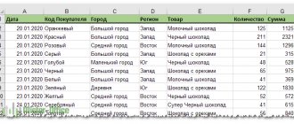
Let there be a source table in the range A 7:C 83 with a list of products, containing the fields (columns) Product, Quantity and Price (see example file). The table should not contain empty rows and columns, otherwise the Advanced filter (and the regular AutoFilter) will not work correctly.
Task 1 (begins...)
Let's set up a filter to select rows that contain values in the Product name starting with the word Nails. This selection condition is satisfied by the rows with the products 20 mm nails, 10 mm nails, 10 mm nails and Nails.
We will place a sign with the selection condition in the range A 1 : A2. The table should also contain the name of the column header by which the selection will be made. As a criterion in cell A2 we indicate the word Nails.
Note : The structure of criteria for the Advanced filter is clearly defined and it coincides with the structure of criteria for the functions BDSUMM(), BCOUNT(), etc.
Typically, Advanced Filter criteria are placed above the table to which the filter is applied, but you can also place them on the side of the table. Avoid placing a sign with criteria under the original table, although this is not prohibited, it is not always convenient, because New rows can be added to the original table.
ATTENTION! Make sure that there is at least one empty line between the table with the values of the selection conditions and the source table (this will make it easier to work with the Advanced filter).
Now everything is ready to work with the Advanced filter:
- select any table cell (this is not necessary, but it will speed up the filling of filter parameters);
- call Advanced filter (Data/Sort and filter/Advanced);
- in the Source range field, make sure that the range of table cells is specified along with the headers ( A 7:C 83 );
- in the Range of conditions field, specify the cells containing the sign with the criterion, i.e. range A 1 :A2 .
If desired, you can copy the selected rows to another table by setting the switch to the Copy result to another location position. But we won't do that here.
Click the OK button and the filter will be applied - only rows containing the names 20 mm nails, 10 mm nails, 50 mm nails and Nails in the Product column will remain in the table. The remaining lines will be hidden.
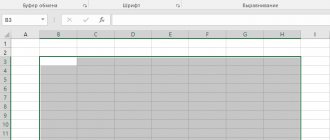
The selected line numbers will be highlighted in blue.
To cancel the filter action, select any table cell and press CTRL+SHIFT+L (AutoFilter will be applied to the header, and the Advanced Filter action will be canceled) or click the Clear menu button ( Data / Sort and Filter / Clear ).
Applying an advanced filter
See also: “How to count the number of characters in an Excel table cell”
So, we have a table with data that needs to be filtered.
To use the advanced filter tool, you need to complete the following steps.
- The first step is to create a second auxiliary table with filter conditions. To create it, you need to copy the header of the source table and paste it into the auxiliary table. For clarity, we will place an additional table at the top, next to the main one. We will also mark it by filling it with a different color (this is done for greater clarity and is not necessary). An auxiliary table can be placed absolutely anywhere in the document, and it is not at all necessary that it be on the same sheet where the main table is located.
- Then we will proceed to filling the auxiliary table with the data that will be required for the work. And we need values from the main table by which we need to filter the data. In our case, we want to select information on female gender and sport – tennis.
- When the auxiliary table is ready, you can proceed to the next step. By placing the cursor on any cell of the initial or auxiliary table, in the main program menu, click on the “Data” tab, select the “Advanced” item from the “Filter” tool block that opens.
- As a result, a window with advanced filter settings should appear.
- This function has two options: “Copy results to another location” and “Filter the list in place”.
As the names suggest, these options control how the filtered information is displayed. In the first option, the data will be displayed separately in the place you specify in the document. In the second - directly in the source table. We select the appropriate option (in our case, we leave the filtering in place) and move on.
- In the “List range” field, you must specify the coordinates of the table (along with the header). This can be done by entering them manually, or by simply selecting the table with the mouse and clicking on the small icon at the end of the field for entering coordinates. In the line “Range of conditions” we indicate the coordinates of the auxiliary table (header and line with conditions) in the same way.
We would like to draw your attention to one important detail. Make sure that there are no empty cells in the selected area. Otherwise, nothing will work. When finished, confirm the specified coordinates by clicking “OK”.
- As a result of these actions, only the data we require will remain in the source table.
- If we select the option “Copy results to another location”, then the result will be output to the location we specified, and the original table will remain unchanged. In this case, in the line “Place result in range” we are required to enter coordinates to display the result. You can specify only one cell, which will be the top-left coordinate for the new table. In this case, the selected cell is A42.
- After clicking the “OK” button, a new table with the specified filtering parameters will be inserted, starting from cell A42.
Problem 2 (exactly the same)
Let's set up a filter to select rows that exactly contain the word Nails in the Product column. This selection condition is satisfied only by rows with the goods nails and Nails (Register is not taken into account). The values 20 mm nails, 10 mm nails, 50 mm nails will not be taken into account.
We will place a sign with the selection condition in the range B1:B2 . The table should also contain the name of the column header by which the selection will be made. As a criterion in cell B2 , we indicate the formula ="= Nails".
Now everything is ready to work with the Advanced filter:
- select any table cell (this is not necessary, but it will speed up the filling of filter parameters);
- call Advanced filter (Data/Sort and filter/Advanced);
- in the Source range field, make sure that the range of table cells is specified along with the headers ( A 7:C 83 );
- in the Range of conditions field, specify the cells containing the sign with the criterion, i.e. range B1 :B2 .
- Click OK
There is no particular point in using the Advanced filter with such simple criteria, because... AutoFilter easily copes with these tasks. Let's look at more complex filtering tasks.
If you specify not ="=Nails" as a criterion, but simply Nails, then all records containing names starting with the word Nails (Nails 80mm, Nails2) will be displayed. To display product lines containing the word nails, for example, New nails, you must specify ="=*Nails" or simply * Nails as a criterion, where * is a wildcard and means any sequence of characters.
How to set advanced search
Advanced search allows you to filter information based on several conditions at once. When working with it, before placing a filter in an Excel table, you need to prepare the table itself - create a field above it from several free lines and copy the headings.
Then, in the free line under the copied headings, set the necessary search conditions. For example, it is necessary to find goods produced in Russia, sold by manager Ivanov, costing less than 300 rubles.
After the parameters have been entered correctly, you must open the “Data” tab again and select the “Advanced” function.
A window will appear in front of the user in which he will have to fill in two lines:
- “Source range” is the range of the table whose information is to be filtered, that is, the source table. Excel will enter it automatically;
- The “range of conditions” are the cells from which the program will take values for elimination - the second table that we created from the top. In order for the values to appear in the window line, you just need to grab two of its lines: with the name of the section and the entered values.
After both ranges are formed, click “Ok” and evaluate the result.
Problem 3 (OR condition for one column)
Let's set up a filter to select rows whose Product column contains a value starting with the word Nails OR Wallpaper.
The selection criteria in this case should be placed under the appropriate column heading (Product) and should be located one below the other in the same column (see figure below). Place the plate with the criteria in the range C1:C3 .
The window with Advanced filter parameters and the table with filtered data will look like this.
After clicking OK, all records containing Nails OR Wallpaper products in the Product column will be displayed.
How to do it right?
How to make an advanced filter in Excel? To make it clear how the procedure occurs and how it is done, let's look at an example.
Instructions for advanced spreadsheet filtering:
- You need to create a space above the main table. The filtering results will be located there. There should be enough space for the finished table. One more line is also required. It will separate the filtered table from the main one.
- In the very first line of the freed space, copy the entire header (column names) of the main table.
- Enter the required filtering data in the required column. Note that the entry should look like this: = "= filtered value".
- Now you need to go to the “Data” section. In the filtering area (funnel icon), select “Advanced” (located at the end of the right list from the corresponding sign).
- Next, in the pop-up window you need to enter the advanced filter parameters in Excel. The Condition Range and Source Range are filled in automatically if the start cell of the worksheet has been selected. Otherwise you will have to enter them yourself.
- Click on Ok. You will exit the advanced filtering settings settings.
After these steps, only records for the specified delimiting value will remain in the main table. To cancel the last action (filtering), you need to click on the “Clear” button, which is located in the “Data” section.
Problem 4 (condition I)
Let's select only those rows of the table that exactly contain products Nails in the Product column, and a value >40 in the Quantity column. The selection criteria in this case should be placed under the appropriate headings (Product and Quantity) and should be located on one line. The selection conditions must be written in a special format: ="= Nails" and =">40". We will place a plate with the selection condition in the range E1:F2 .
After clicking the OK button, all records containing Nails products with a quantity >40 in the Product column will be displayed.
TIP: When changing selection criteria, it is better to create a table with the criteria each time and, after calling the filter, just change the link to them.
Note : If you had to clear the Advanced filter parameters (Data/Sorting and Filter/Clear), then before calling the filter, select any table cell - EXCEL will automatically insert a link to the range occupied by the table (if there are empty rows in the table, a link will be inserted not to the entire table, but only up to the first empty line).
Custom sorting
But, as we see, with these types of sorting by one value, data containing the names of the same person are arranged within the range in random order.
But what if we want to sort names alphabetically, but for example, if the name matches, make sure that the data is arranged by date? To do this, as well as to use some other features, all in the same “Sorting and Filter” menu, we need to go to the “Custom sorting...” item.
After this, the sorting settings window opens. If your table has headers, then make sure that in this window there is a checkmark next to the “My data contains headers” option.
In the “Column” field, indicate the name of the column by which the sorting will be performed. In our case, this is the “Name” column. The “Sorting” field indicates what type of content will be sorted by. There are four options:
- Values;
- Cell color;
- Font color;
- Cell icon.
But, in the vast majority of cases, the “Values” item is used. It is set by default. In our case, we will also use this particular point.
In the “Order” column we need to indicate in what order the data will be arranged: “From A to Z” or vice versa. Select the value “From A to Z”.
So, we have set up sorting by one of the columns. In order to configure sorting by another column, click on the “Add level” button.
Another set of fields appears, which must be filled in to sort by another column. In our case, according to the “Date” column. Since the date format is set in these cells, in the “Order” field we set the values not “From A to Z”, but “From old to new”, or “From new to old”.
In the same way, in this window you can configure, if necessary, sorting by other columns in order of priority. When all settings are completed, click on the “OK” button.
As you can see, now in our table all the data is sorted, first of all, by employee names, and then by payment dates.
But that's not all the possibilities of custom sorting. If desired, in this window you can configure sorting not by columns, but by rows. To do this, click on the “Options” button.
In the sorting options window that opens, move the switch from the “Range Rows” position to the “Range Columns” position. Click on the “OK” button.
Now, by analogy with the previous example, you can enter data for sorting. Enter the data and click on the “OK” button.
As you can see, after this, the columns have swapped places, according to the entered parameters.
Of course, for our table, taken as an example, using sorting by changing the location of the columns is not particularly useful, but for some other tables this type of sorting can be very appropriate.
Problem 5 (OR condition for different columns)
The previous problems could, if desired, be solved using a regular autofilter. The same problem cannot be solved with a conventional filter.
Let's select only those table rows that exactly contain Nails products in the Product column, OR that contain a value >40 in the Quantity column. The selection criteria in this case should be placed under the appropriate headings (Product and Quantity) and should be located on different lines. The selection conditions must be written in a special format: =»>40″ and =»= Nails». We will place the plate with the selection condition in the range E4:F6 .
After clicking the OK button, records will be displayed containing products Nails OR a value >40 (for any product) in the Product column.
How to use a filter in Excel
Immediately after turning on the filter, the table will not change (not counting the arrows that appear in the column headers). To filter some of the data you need, click on the arrow in the column you want to filter on. In practice it looks like the figure below.
Meaning of the filter:
is that Excel will leave only those table rows that in THIS (with the configured filter) column contain a cell with the selected value. Other lines will be hidden.
To remove filtering (without deleting the filter!) simply check all the boxes. The same effect will occur if you remove the filter completely - the table will again take its original form.
Task 6 (Selection conditions created as a result of applying the formula)
The real power of the Advanced Filter comes into play when you use formulas as filter criteria.
There are two options for setting row selection conditions:
- directly enter values for the criterion (see tasks above);
- form a criterion based on the results of the formula.
Let's consider the criteria specified by the formula. The formula specified as the selection criterion must return TRUE or FALSE.
For example, let's display rows containing a Product that appears in the table only once. For this:
- enter the formula in cell H2 =COUNTIF(Sheet1!$A$8:$A$83,A8)=1
- in H1, instead of the title, we will enter explanatory text, for example, Non-repeating values. Explanatory text must NOT match any table column heading! Otherwise the filter will not work properly.
H1:H2 as the range of conditions .
Note that the range of search values is entered using absolute references, and the criterion in the COUNTIF() function is entered using relative reference. This is necessary because when you apply the Advanced Filter, EXCEL will see that A8 is a relative reference and will move down the Product column one entry at a time and return either TRUE or FALSE. If TRUE is returned, the corresponding table row will be displayed. If FALSE is returned, the row will not be displayed after applying the filter.
TIP: To test whether the formula works, you can create an additional column next to the table (for example, in F) and enter the above formula in cell F8, and then copy it down. A TRUE/FALSE column will be generated that will help you determine how your formula works.
Examples of other formulas from the example file:
- Display rows with prices greater than the 3rd highest price in the table. =C8>LARGEST($С$8:$С$83,5) This example clearly shows the insidiousness of the MAXIMUM() function. If we sort column C (prices), we get: 750; 700; 700 ; 700; 620, 620, 160, ... In human understanding, the “3rd highest price” corresponds to 620, and in the understanding of the HIGHEST() function – 700 . As a result, not 4 lines will be displayed, but only one (750);
- Outputting strings with CASE sensitivity = COINCIDENT("nails";A8) . Only those lines in which the product nails is entered using lowercase letters will be displayed;
- Displaying rows whose price is higher than average =С8>AVERAGE($С$8:$С$83) ;
ATTENTION! Applying an Advanced Filter cancels the filter applied to the table (Data/Sort & Filter/Filter).
How to put
Excel is a powerful Microsoft program designed to work with tables.
It is convenient to keep a large record of a lot of data. And regularly, users have a need to quickly find in files with thousands of data those that meet a certain parameter. To do this, you will have to put a filter in the Excel table. To get started, you need to select one, any, cell inside the table, open the “Data” tab.
Then click the “Filter” button.
Unused dropout icons will appear in the column headers. This means that all that remains is to set the necessary parameters to cut off the necessary information.
In the table
Step-by-step instructions: how to add a filter to an Excel table.
1. Click on the icon in the column header.
The user will see a drop-down window listing all the values in this column.
2. Remove unnecessary checkmarks from parameters that the user is not interested in. Checkmarks will remain only for those parameters that need to be searched. Then click “Ok”.
3. View the result - only rows corresponding to the specified parameter will remain.
In the range
Screening in a range is used when it is necessary to cut off information not according to one value, but along a certain spectrum. It can be numeric or text, depending on the information that the required column contains.
For example, in the file in question, columns B and C have numeric screening.
The rest are text.
To set up a range search, you need to click the icon in the column header, select the line with the name of the dropout and the required method for setting the range, set it and apply.
For example, in the case of numerical search, this procedure looks like this:
1. Select the type of screening.
2. Select the required method for forming the range, for example, “greater than” means that the result will be all values greater than the number that the user enters.
3. Enter a number, which will become the cutoff limit; all values greater than it will be displayed.
4. Click “Ok” and evaluate the result. Only values that exceed the specified limit will remain in the selected column.
Task 7 (Selection conditions contain formulas and usual criteria)
Let's now consider another table from the example file on the sheet Task 7.
The Product column shows the name of the product, and the Product Type column shows its type.
The task is to display products for a given type of product whose price is below the average. That is, we have 3 criteria: the first criterion specifies the Product, the 2nd – its Type, and the 3rd criterion (in the form of a formula) specifies the price below the average.
We will place the criteria in lines 6 and 7. Enter the required Product and Product Type. For a given Product Type, we calculate the average and display it for clarity in a separate cell F7. In principle, the formula can be entered directly into the criterion formula in cell C7. The explanatory text in the cell above the formula (C6) should NOT match any table column heading! Otherwise the filter will not work properly.
Next, we proceed as usual: select any table cell, call the Advanced Filter and specify a range with criteria.
2 products out of 4 (of the given product type) will be displayed.
In the example file, for convenience, Conditional formatting is used: rows that satisfy the first 2 criteria are selected (for more details, see the article Selecting table rows in MS EXCEL depending on the condition in the cell).
What is this function? Description
What does advanced filter mean in Excel? This is a function that allows you to differentiate selected data (by columns in Excel) relative to the entered requirements.
For example, if we have a spreadsheet with information about all the students of the school (height, weight, class, gender, etc.), then we can easily identify among them, say, all the boys with a height of 160 from the 8th grade class. You can do this using the Advanced Filter feature in Excel. We will talk about it in detail further.
Problem 7.1. (Are the 2 values on the same line the same?)
There is a table that shows the year of manufacture and year of purchase of the car.
You want to display only those rows in which the Year of Manufacture coincides with the Year of Purchase. This can be done using the elementary formula =B10=C10.
The explanatory text in cell C6 must NOT match any table column heading! Otherwise the filter will not work properly.
Drawing up a table of conditions
First of all, we need to create a condition table in accordance with our task:
Conditions are built in rows, which consist of fields (columns). The headings of the condition table must exactly match the headings of the source range.
Please note that the “Window Date” field. contract" is repeated. This means that both conditions must be met for the filter to pass the data. It is also possible to use formulas (shown in the image) and wildcards to create filtering rules.
Problem 8 (Is the symbol a number?)
Let's say we have a table listing different types of nails.
You want to filter only those rows that have 1" Nails, 2" Nails, etc. in the Product column. products Stainless steel nails, chrome plated nails, etc. should not be filtered.
The easiest way to do this is to set the condition as a filter that after the word Nails there should be a number. This can be done using the formula =ISNUMBER(—PSTR(A11,LENGTH($A$8)+2,1))
The formula cuts out 1 character from the product name after the word Nails (including the space). If this character is a number (digit), then the formula returns TRUE and the string is printed, otherwise the string is not printed. Column F shows how the formula works, i.e. it can be tested before running the Advanced Filter.
Why do we need filters in Excel tables?
And then, to be able to quickly select only the data you need, hiding unnecessary rows . Thus, the filter allows you without deleting rows in an Excel table.
Table rows hidden by a filter do not disappear. You can roughly imagine that their height becomes zero (I previously talked about changing the height of rows and width of columns). Thus, the remaining lines that are not hidden by the filter are, as it were, “glued together.” What comes out as a result is a table with a filter applied.
Externally, a table with a filter in Excel looks the same as any other, but at the top of it, special arrows appear in each column. You can see an example of a table with a filter applied in the picture below.
Now let's see how to actually add filters to the table.
Task 9 (Output rows that DO NOT CONTAIN the specified Products)
You need to filter only those rows that do NOT contain in the Product column: Nails, Board, Glue, Wallpaper.
To do this, you will have to use a simple formula =END(VLOOKUP(A15,$A$8:$A$11,1,0))
The VLOOKUP() function searches in the Product column of each row for the names of products specified in the range A8:A11 . If these products are NOT found, VLOOKUP() returns the #N/A error, which is processed by the END() function - as a result, the formula returns TRUE and the line is printed.