Line wrapping is a great technique for improving the appearance of long text in a cell. This allows you to fit more information inside it without increasing the width of the column.
The standard method for adding line breaks to a cell is to use the Alt + Enter key combination. This has become widespread. All this looks beautiful, but to a certain extent impractical. After all, these tables have not yet worked, and this poses additional difficulties.
In some cases, such a transfer is added automatically when text is copied from other programs. And this could already become a problem. However, if you know a few tricks, you can make your life a lot easier.
Symbol function
If you need to enter a large amount of data regularly, it is much better to automate adding line breaks than to press the above key combination every second.
To do this you can use the SYMBOL
, which allows you to insert any ASCII character into a cell. But before describing how to use it, you need to understand how it works.
Excel uses different character codes all the time. Each letter and icon has its own code from 1 to 255. For example, the code of the capital letter A is 97. The line break is numbered 10. And although this symbol is invisible, it helps the program understand where to hyphenate. Therefore it is very important.
Before you can wrap a line, you must enable the “Text Wrap” mode. This way you can make sure that the line break character is not visible.
When a wrap is added to a histogram, graph, or chart, line breaks naturally occur. That is, with its help you can divide one line into two or more, not even in cells, but in absolutely any other Excel object.
Video to help
It is often necessary to wrap text inside one Excel cell to a new line. That is, move the text along the lines inside one cell as indicated in the picture. If, after entering the first part of the text, you simply press the ENTER key, the cursor will be moved to the next line, but to a different cell, and we need a transfer in the same cell.
This is a very common task and it can be solved very simply - to move text to a new line inside one Excel cell, you need to press ALT+ENTER (hold down the ALT key, then without releasing it, press the ENTER key)
Removing line breaks
As mentioned above, if you add line breaks, these invisible characters can cause a lot of inconvenience. But with the right approach, you can figure out how to get rid of them.
Since you already know that adding line breaks is possible using the Ctrl + Enter combination, you will still have to figure out how to eliminate them if there are additional characters. After all, no one will deny that it is impossible to start without the ability to brake. Therefore, being able to remove line breaks is very important.
Of course, you can try to perform this operation manually, deleting rows one by one. But if there are too many of them, it will take a lot of time and require a lot of effort.
So what can you do to automate the process of removing line breaks? This can be done in several ways.
Replacing the hyphen character
The easiest way to remove hyphenation is to use Excel's standard Find and Replace function. You need to select all the cells available in the document by pressing the key combination Ctrl + A and bringing up the corresponding dialog box using the key combinations Ctrl + H. You can also open the Find and Replace window from the Home tab of the ribbon where you will find and select the Search group and click the Replace button.
Here the attentive and thoughtful reader will have a question: what should you enter in the top “Search” field if the symbol is invisible and is not on the keyboard? And here it is not possible to enter the "Alt + Enter" key combination, so you cannot copy it from the finished table.
But this combination has an alternative - Ctrl + J. This key combination can replace Alt + Enter in any dialog box or input field.
After the user adds a blinking cursor to the Find field and enters the Ctrl + J key combination, nothing visually changes. This should not be confusing, since the symbol itself is invisible, and even if the Excel user wants, it cannot be detected.
You can leave nothing in the “Replace” field. If you want the lines not to be connected, you can put a space. As a result, there will be free space between the lines. To confirm the action, you need to click the “Replace All” button. That's it, after this transfer there will be no transfer throughout the entire document.
Fair and reverse move. If you enter a space in the Find field and press Ctrl + J in the Replace field, all spaces will be replaced with line breaks. This can be very convenient in some situations. For example, if there is a list of words that were accidentally printed in a row, while they should be put in a column. In this case, you can open the same Find and Replace window and replace the space with a line break.
It is important to consider one more point. The newline character entered in the Find field may remain after being replaced when this dialog box is opened a second time. Therefore, it is better to call it again and press the “Backspace” button several times, and the cursor will be placed in the field.
Formula for removing line breaks
If you need to use a formula only to remove line breaks, you should use the PECHCHIM
, designed to remove all invisible characters. Line breaks are no exception.
But this option is not always suitable because after removing the line breaks they may stick together, so it is better to use another formula that will replace the line break with a space.
To do this, use a combination of functions SYMBOL
and
SUBSTITUTE
. The first returns the character by code, and the second replaces the character with other text. In most cases, line breaks should be replaced with spaces, but you can also replace them with commas.
Method 2: Transfer via Insert
See also: “INDEX function in Excel: examples, use with SEARCH”
Using the paste method makes it much easier and faster to change the location of rows compared to the copying method described earlier. Let's look at the functionality of this method using the table from the first method as an example.
- On the vertical coordinate panel we find the number of the required line, click on it with the left mouse button. This action resulted in the allocation of the entire deadline. Find the “Clipboard” block in the tool ribbon, which is located in the “Home” tab, and select “Cut” (the scissors icon). You can also use the context menu (called by right-clicking on the selected fragment) in which we select the appropriate “Cut” item.
- Now we right-click on the coordinate panel on the number of the line above which we want to place the data cut out in the first stage. In the context menu that appears, select “Insert cut cells.”
- As a result, the desired line moved to the selected location, while the remaining lines retained their sequence.
This method involves performing only three simple and understandable steps, which significantly saves the user’s time and effort. But using the appropriate tools and launching the context menu slows down the process of changing the location of rows in the table. Therefore, let’s move on to analyzing the fastest way to solve the problem assigned to us.
Division into columns by line breaks
The Text to Columns tool, located in the Data tab, also works well with line breaks. To do this, in the second step, select the “Other” separator and enter a newline character using the key combination Ctrl + J.
If the table has multiple line breaks one after the other, check the “Count consecutive delimiters as one” checkbox. And after you click the Next button, we will get this result.
Attention! Before you begin this operation, you must insert as many columns without values as possible into the cells to the right of the shared column so that the resulting text does not exclude the contents of the cells to the right of those in which the line break works.
Important Note
Please note that in order for text to be correctly wrapped across different lines, you must enable the Wrap Text .
Otherwise, even if the text in the formula bar is written on different lines, the cell will be displayed as one, since the text wrapping property was not enabled.
Thank you for your attention! If you have thoughts or questions on the topic of the article, write and ask in the comments.
Good luck to you and see you soon on the pages of the TutorExcel.Ru blog!
Share with friends:
How to split text into multiple lines?
Excel gives you the ability to divide text that consists of several lines into separate lines.
It is quite problematic to achieve this goal on your own. You can use a macro to automate a task. To do this, however, you must learn programming skills. Not everyone needs this, since the use of macros is necessary only for those who devote a lot of time to spreadsheets and have to spend a lot of time on them. But the average user does not work only with Excel; he has many other programs.
But how can you do without programming skills if you still have to constantly split lines? The easiest way is to use Power Query.
Description of the Power Query add-in
This add-in was included by default in Excel 2020 for the first time. However, if you are using an older version, you can download it from the Microsoft website. Power Query is an addon that allows you to connect to various data and process it for further analysis. It can also be used to separate strings.
To load data into Power Query, you must convert it to Smart Table format. To do this, press the key combination Ctrl + T or click the “Format” button, as in the table on the “Home” tab. But if you don't want to do this, there is a way to do it differently.
If you want to work with "dumb" tables, you can simply select the source record and give it a name in the "Formulas - Name Manager - Create" tab.
Next, on the “Data” tab (in Excel versions starting from 2020) or on the Power Query tab (if Excel is an older version with the add-on installed), click on the “From table/range” button to transfer the data to the Power Query editor.
After the data is loaded, the column with multi-line text is highlighted, and on the “Home” tab, find the option “Split column – By delimiter”.
It's likely that Power Query will independently determine what criteria the split should be based on, and will itself place the # (lf) line break character so that the user can see where that invisible character is. If necessary, you can use other characters selected from the drop-down list located at the bottom of the window after selecting the "Split using special characters" checkbox.
To ensure that data is split into rows rather than individual columns, you must enable the appropriate selector in the advanced options group.
All that remains is to confirm the settings by pressing the OK button and get the desired result.
The resulting table can be inserted into a worksheet using the command “Close and load” – “Close and load into...”. You can find it on the Home tab.
Note that Power Query requires data to be refreshed after every change because there is no input for formulas. To do this, right-click the table and select Refresh from the drop-down menu. Or you can find the Refresh button on the Data tab.
Method 3: Move with the Mouse
Thanks to this method, you can transfer data to a new location as quickly as possible. For this, only the mouse and keyboard are used. Let's look at how it all works.
- On the coordinate panel, left-click on the number of the line that we need to move.
Place the cursor over the top border of any cell in the selected row, and it should transform into an arrow with pointers in four different directions. Hold down the Shift key on the keyboard and move the line to any place we need using the left mouse button held down. Please note that if the Shift button is not pressed, then data will be replaced instead of transferred, and confusion will arise in the table.
Using a macro to split a line
Macros are a convenient method for automating any workflow in Excel. Although it offers great possibilities to those who use it, this tool requires a very intensive learning curve as it involves programming.
To use a macro to separate lines with breaks, you must go to the “Developer” tab or press the Alt + F11 combination. Then a window will open in which a new module is inserted through the “Insert – Module” menu. Then you need to copy this code and paste it into the Visual Basic development environment.
Sub Split_By_Rows()
Dim cell As Range, n As Integer
Set cell = ActiveCell
For i = 1 To Selection.Rows.Count
ar = Split(cell, Chr(10))
'split the text into an array
n = UBound(ar)
'determine the number of fragments
cell.Offset(1, 0).Resize(n, 1).EntireRow.Insert
' insert empty lines below
cell.Resize(n + 1, 1) = WorksheetFunction.Transpose(ar)
'enter data from the array into them
Set cell = cell.Offset(n + 1, 0)
'shift to the next cell
Next i
End Sub
Method 4
To move text in a cell, another formula is used - CONCATENATE(). Let's take only the first line with the headings: Last Name, Debt, Payable, Amount. Click on an empty cell and enter the formula:
=CONCATENATE(A1,CHAR(10),B1,CHAR(10),C1,CHAR(10),D1)
Instead of A1, B1, C1, D1, indicate the ones you need. Moreover, their number can be reduced or increased.
The result we will get is this.
Therefore, open the already familiar Format Cells window and mark the transfer item. Now the necessary words will begin on new lines.
In the next cell I entered the same formula, only I indicated other cells: A2:D2.
The advantage of using this method, like the previous one, is that when the data in the source cells changes, the values in these will also change.
In the example, the debt number has changed. If you also automatically calculate the amount in Excel, then you won’t have to change anything else manually.
How to remove line breaks using a macro?
If line breaks were added by mistake or appeared there after copying information from another source, you can use a macro to remove them.
The advantage of this method of removing line breaks is that you only need to create it once, and then they can be used with any workbook.
Disadvantage - as in the previous example, programming skills are required.
Simply paste the following code into the Visual Basic editor.
Sub RemoveCarriageReturns()
Dim MyRange As Range
Application.ScreenUpdating = False
Application.Calculation = xlCalculationManual
For Each MyRange In ActiveSheet.UsedRange
If 0 < InStr(MyRange, Chr(10)) Then
MyRange = Replace(MyRange, Chr(10), “”)
End If
Next
Application.ScreenUpdating = True
Application.Calculation = xlCalculationAutomatic
End Sub
How to wrap text in a cell in Excel
If you periodically create documents in Microsoft Excel, then you will notice that all data entered into a cell is written on one line.
Since this may not always be suitable, and the option to stretch the cell is also not appropriate, the need arises to wrap the text.
The usual “Enter” press is not suitable, since the cursor immediately jumps to a new line, so what should I do next?
In this article, we will learn how to move text in Excel to a new line within one cell. Let's look at how this can be done in various ways.
- Method 1
- Method 2
- Method 3
- Method 4
- Method 5
Method 1
You can use the key combination “Alt+Enter” for this. Place italics in front of the word that should start on a new line, press “Alt”, and without releasing it, click “Enter”. Everything, italics or phrase will jump to a new line. Type all the text in this way, and then press “Enter”.
The bottom cell will be selected, and the one we need will increase in height and the text in it will be fully visible.
To perform some actions faster, check out the list of shortcut keys in Excel.
Method 2
To ensure that while typing words, italics automatically jump to another line when the text no longer fits in width, do the following. Select a cell and right-click on it. In the context menu, click Format Cells.
At the top, select the “Alignment” tab and check the box next to “word wrap”. Click "OK".
Write everything you need, and if the next word does not fit in width, it will start on the next line.
If in a document lines must be wrapped in many cells, then first select them, and then check the box mentioned above.
Method 3
In some cases, everything that I described above may not be suitable, since it is necessary that information from several cells be collected in one, and already divided into lines in it. So let's figure out what formulas to use to get the desired result.
One of them is SYMBOL(). Here, in brackets, you need to indicate a value from one to 255. The number is taken from a special table, which indicates which character it corresponds to. To move a line, code 10 is used.
Now about how to work with the formula. For example, let's take data from cells A1:D2 and write what is written in different columns (A, B, C, D) in separate lines.
I put italics in the new cell and write in the formula bar:
=A1&A2&CHAR(10)&B1&B2&CHAR(10)&C1&C2&CHAR(10)&D1&D2
We use the “&” sign to concatenate cells A1:A2 and so on. Press "Enter".
Don't be afraid of the result - everything will be written in one line. To fix this, open the “Format Cells” window and check the transfer box, as described above.
As a result, we will get what we wanted. The information will be taken from the indicated cells, and where CHAR(10) was entered in the formula, a transfer will be made.
Method 4
To move text in a cell, another formula is used - CONCATENATE(). Let's take only the first line with the headings: Last Name, Debt, Payable, Amount. Click on an empty cell and enter the formula:
=CONCATENATE(A1,CHAR(10),B1,CHAR(10),C1,CHAR(10),D1)
Instead of A1, B1, C1, D1, indicate the ones you need. Moreover, their number can be reduced or increased.
The result we will get is this.
Therefore, open the already familiar Format Cells window and mark the transfer item. Now the necessary words will begin on new lines.
In the next cell I entered the same formula, only I indicated other cells: A2:D2.
The advantage of using this method, like the previous one, is that when the data in the source cells changes, the values in these will also change.
In the example, the debt number has changed. If you also automatically calculate the amount in Excel, then you won’t have to change anything else manually.
conclusions
Dividing a row allows you to make working with Excel tables more convenient. And using the above techniques, you can do it at a professional level.
You also learned how to remove line breaks if necessary.
We see that there are many different methods for adding and removing line breaks. At first glance, it even seems incredible that all these functions are needed and there is no surplus. But it all comes down to how often spreadsheets are used.
Thank God, Excel’s functionality is so wide that you can use it to implement absolutely any idea that comes to mind.
Rate the quality of the article. Your opinion is important to us: