Microsoft Office Excel is a data editing program. The information in the file is presented in the form of a table, which consists of rows and columns. The smallest unit of measurement in an Excel document is the cell. These elements are numbered based on their relationship to the column and row, such as A1 or D13. You can change the width and height of the cells to give them the look you want so that the shape, size and aspect ratio fit your requirements. In addition, you can merge adjacent elements on either side or undo the division to customize table structures. Unfortunately, since a cell is the smallest file unit in Excel, you cannot split it.
Excel spreadsheets are very popular and are often used to work with data. Sometimes users need to divide a cell into two or more parts, but the program does not have such an option. However, there are ways to get around this limitation and give the table the look you want.
The need to split a cell may arise if one of the columns must contain two or more data elements. For example, two or more names of a certain item, while others in the “name” column have only one. In addition, some users need to split the data contained in one cell into several. The most common example is dividing a person’s full name separately into last name, first name and patronymic, so that each value occupies a separate cell. In both cases, you can perform the division using features such as Cell Merge, Text to Columns, Flash Fill, and a variety of formulas that are customized for each case.
How to Split a Cell in an Excel Spreadsheet Using Outline Planning
Excel has a certain table structure - this is necessary to make it easier to navigate the data, and also to avoid errors in formulas and calculations, problems with combination and reading. Each cell has its own individual number, which is determined by its position on the axes of numbers and Latin letters. For example, the alphanumeric address of the first element in the table is A1. One row corresponds to one table cell, and vice versa. This means that it is a minimal element and cannot be divided into two or more independent ones.
In some cases, an Excel user needs to make sure that one column has two or more values to intersect with one of the rows. For example, in the case when a particular thing has several names or numbers, and the data of the rest fits into one cell. Similarly with rows, if one column includes primary categories (for example, “programmers”, “designers” and so on), and the other contains secondary categories (“programmers” - Ivan, Peter). Although you can't do this directly in the editor, you can work around the limitation. To do this you need:
- Plan in advance what the maximum number of values will include in a row or column;
- At the stage of preparing the Excel sheet for work, combine those cells of a column or row that will be used as single cells;
- Thus, “divided” cells will represent independent elements, and “whole” cells will be connected, that is, the result will be visual (but it will still meet Excel requirements).
Example: in column A and rows 1–5 you have 5 last names, and the adjacent column B contains the positions of these people in the company. If one or more people hold 2 positions, enter the second one in column C, and for the rest, simply combine B1 and C1, B2 and C2, and so on. Similarly in cases where one value in the first column corresponds to more than 2 in subsequent ones. Each cell will have its own address in Excel and will remain fully functional.
Method 3: Drawing by yourself
There is another method for dividing cells in a Word table, which, unlike the previous two, allows you to do this not only strictly symmetrically, but also arbitrarily, by manually drawing a line that will divide the element into columns and/or rows.
- Go to the “Insert” tab, click on the “Table” button and select “Draw Table”.
Note: You can call the same tool through the “Layout” tab by first selecting the entire table or clicking on any part of it.
- The cursor pointer will change to a pencil, with which we will split the cell.
To do this, it is enough to draw a vertical or horizontal line in it (be sure to do this strictly from border to border and as evenly as possible), depending on whether you need to make rows or columns.
If desired, you can divide the cell into both rows and columns.
- It’s easy to guess that this tool allows you to divide a cell into an unlimited number of elements.
In addition, you can draw a border not only in one of them, but also in several at once.
We previously wrote about all the nuances of independently drawing tables in a separate article.
Read more: How to draw a table in Word
We are glad that we were able to help you solve the problem. Add the Lumpics.ru website to your bookmarks and we will be useful to you. Thank the author and share the article on social networks.
Describe what didn't work for you. Our specialists will try to answer as quickly as possible.
How to split cells merged when planning a structure
If, after actions similar to those described in the previous paragraph, you decide that the entire page needs to be returned to its previous state and split cells:
- Open the desired sheet, select all the cells (or a specific part) and go to the “Home” tab on the top panel of Excel;
- In the Alignment area, click the arrow and open the drop-down list with the Merge and Center options, then select Unmerge Cells;
- The elements will be split into single elements, but all the data will be shifted to the upper left - you can distribute them across columns using the “Text by Columns” function, which we will look at next.
Content
- 1 Example 1. Divide text with full name into columns using formulas
- 1.1 Let's start dividing the first part of the text - Surnames
- 1.2 Let's start dividing the second part of the text - Name
- 1.3 Let's start dividing the third part of the text - Patronymic
- 2 Example 2. How to split text into columns in Excel using a formula
Example 1. We divide text with full name into columns using formulas If we look at the example of dividing full name, then we can divide the text using Excel text formulas using the PSTR and FIND functions, which we discussed in previous articles.
In this case, you just need to insert data into a specific column, and the formulas will automatically split the text as you need. Let's start looking at this example. We have a column with a list of full names, our task is to place the last name, first name and patronymic in separate columns.
Let's try to describe the action plan in great detail and divide the solution to the problem into several stages. First of all, we’ll add auxiliary columns for intermediate calculations to make it clearer for you, and at the end we’ll combine all the formulas into one.
So, let's add columns position 1st and 2nd spaces. Using the FIND function, as we already discussed in the previous article, we will find the position of the first space. To do this, in cell “H2” we write the formula
=FIND(" "-A2-1)
and pull it down. Now we need to find the sequence number of the second space. The formula will be the same, but with a slight difference. If we write the same formula, the function will find us the first space, but we need the second space.
This means that it is necessary to change the third argument in the FIND function - the starting position - that is, the position from which the function will search for the searched text.
We see that the second space is in any case after the first space, and we have already found the position of the first space, which means by adding 1 to the position of the first space we will tell the FIND function to look for the space starting from the first letter after the first space.
The function will look like this:
=FIND(" "-A2-H2+1)
Next, we stretch the formula and get the positions of the 1st and 2nd spaces.
How to visually split a cell in an Excel table, how to split an element diagonally
If you just need to split a cell visually without changing its properties and addresses in Excel, you need to:
- Place the cursor on the required element or select several (or the entire sheet).
- Open the “Home” tab, in the “Cells” area, click “Format”.
- A drop-down menu will open where you need to select “Format Cells”.
- In the new window, you need to go to the “Border” tab - here you can draw the necessary cell frames yourself (vertical, horizontal and diagonal lines, several line options and many colors).
- There is another option - you need to right-click on the selected cells to bring up the context menu, then select “Format Cells”, go to the “Border” tab and make lines in the same way.
- One or more selected cells will receive the layout you specified.
In order to make a cell that will include the names of rows and columns at the same time, you need to do:
- In the “Format Cells” window, in the “Border” tab, draw any diagonal line that goes from the upper left to the lower right corner.
- Apply formatting.
- Enter text in the “top” of the cell (it is divided only visually) that will correspond to the line, for example, “title”).
- Align it to the left or right, position it more precisely using spaces.
- While editing an item, press Alt + Enter to go to a new line, then enter text for the column, for example, "quantity";
- If the text is not positioned or looks the way you want, you may need to reposition it using a space bar or change the size and aspect ratio of the cells.
Method 1: Context Menu
The simplest way to separate cells in a Word table is to access the context menu called up on the corresponding element.
Important! If a cell contains data, it will end up being placed in the first cell - left, top, or top left, depending on how and how many elements the division is made into.
- Right-click (RMB) on the cell that you want to “split”.
- Select "Split Cells".
- In the window that appears, indicate the “Number of columns” and “Number of rows” that you want to receive in this table element. Click "OK" to confirm.
Note: To split vertically, you must specify the number of columns, and horizontally, the number of rows. The example below shows one cell divided vertically into two, so it now has two columns. The number of elements obtained as a result of this action is not limited, but it is worth considering their future size and the amount of data that will need to be entered.
If you made a mistake when dividing cells, either use the “Ctrl+Z” keys to undo the action, or select the table elements resulting from the division, call the context menu and select “Merge Cells”.
How to split cell data into Excel table columns using a separator
If you have cells that are filled with some data and need to be categorized into columns, use the split feature. It is perfect when the elements contain information, for example, about the invited people - first name, last name, ticket number, their city or country, date of arrival. If all this was transferred from a text document, it will have no formatting. To make it more convenient to work in Excel, the data needs to be divided into the appropriate columns - “first name”, “last name” and so on.
This is done like this:
- Create new empty columns if there are not enough of them to the right of the one that contains information (there should be no less than the number of data categories), otherwise the information will be written to others that are already filled. Place the mouse cursor after the desired column on the line with Latin letters and click on the table frame with the right mouse button, select “Insert” in the context menu. If you need to add several empty columns, first select a similar number to the right of the one you are looking for (click on the cell with the Latin letter and drag the selection).
- Select the column you want to split. Open “Data” - “Working with data” - “Text by columns”.
- In the new window (Wizard for distributing text into columns), select a data format. If the column you are looking for contains information of different categories separated by spaces or commas, select “Delimited”, if it has a fixed amount of data - “Fixed width” (for example, a digital identifier - we will look at this option later), click “Next”.
- Then specify the delimiters that are used in the array of text in the column. List them in the “Separator character is” (if there is more than one, list them all in the “Other” field). Also specify “Count consecutive delimiters as one” if the data contains several types in a row (for example, two spaces in a row or a period that indicates an abbreviation of a word, and not the end of a sentence, and is followed by a comma).
- Set up a line delimiter if the text contains sentences that are highlighted in quotation marks and contain delimiters from another paragraph, but cannot be split. These include sentences like “Russia, Moscow” - the address in this case must remain intact. If you don't set a limiter, "Russia" and "Moscow" will end up in different columns.
- Select a data format. By default it is "General". If your information contains dates or amounts of funds, indicate the appropriate columns in which they will be placed. Here you can also specify where certain data will be placed. Click on the range selection icon to the right of “Place in” and select the leftmost free column to be filled as the first column. Unfortunately, the data cannot be moved to another Excel workbook or even to another sheet, but you can split it on the current one, and then simply copy it to the desired location.
- Click "Done" - all settings will be applied. Save the document so you don't lose them.
Merge and split cells and tables
⇐ PreviousPage 8 of 28Next ⇒To merge cells :
· select the cells that need to be merged;
· in the Table , select the Merge Cells command.
To split a cell :
· select the cell you want to split;
· in the Table , execute the command Split cells ;
· a dialog box will appear, in it indicate the number of cells into which you want to split the selected cell and click on the OK .
To split the entire table :
· place the cursor in the table;
· in the Table , execute the Split table command.
Work order
1. Open the file used in Lab 5.
2. Create a table and fill it with data from the list of students in your group.
3. Insert a table title.
4. Add one line at the beginning, middle and end of the table.
5. Increase and then decrease the row height.
6. Add one column at the beginning, middle and end of the table.
7. Reduce the width of the added columns.
8. Select all added columns at once.
9. Remove added columns.
10. Using Tables and Borders , create a table.
11. Using the AutoFormat , change the table view.
12. Merge and then split cells.
13. Split the table, and then convert the resulting text back into a table.
14. As instructed by the teacher, draw and fill out a table whose columns contain different numbers of cells.
15. Save the file under the same name.
Contents of the report
1. Purpose of the work.
2. Brief description of the progress of laboratory work.
3. Written answers to test questions as directed by the teacher.
6.4 Security questions
1. How and in what ways can you create a table?
2. How can you increase or decrease the number of columns and rows?
3. How can I increase and how can I decrease the column width?
4. How can I increase and how can I decrease the line height?
5. How can you change a table using the AutoFormat function?
6. How is the Tables and Borders ?
7. How can you select a cell, row, column?
8. How can you select multiple adjacent cells or multiple non-adjacent columns or rows?
9. How can you select the entire table?
10.How can you select multiple non-adjacent cells, multiple non-adjacent columns or rows?
11.How can you merge and split cells?
12.How to convert text into a table?
LABORATORY WORK No. 7
FORMULA EDITOR. DRAWINGS. PRINTING A DOCUMENT
Purpose of work : learn to create formulas, drawings, and print documents in Word.
Theoretical information
Formula editor
To create formulas, there is a special formula editor Microsoft Equation . Sometimes it has to be installed in addition to the Word program. To open the formula editor, select the Object... Insert and select Microsoft Equation Insert Object . You can also use the button on the formatting bar. If this button is not on the panel, you can insert it yourself. To do this, in the Tools select the Settings... , on the Commands Insert category on the left , find the Formula Editor and holding it with the left mouse button, drag it to the panel, Figure 7.1.
Figure 7.1 — Selecting the Formula Editor
Formula toolbar contains more than 150 mathematical symbols. The bottom row is used to select a variety of templates for constructing fractions, integrals, sums, and other complex expressions.
Figure 7.2 — Formula
Write the formula starting from its left side, select the necessary symbols on the toolbar (∑ ÷ ± ≥, etc.), and enter variables and numbers from the keyboard. To move to the beginning or end of the formula, use the cursor keys.
Examples of formulas: ; .
Note : in the editor you should type the entire formula, not just its right side. If you need to change an already typed formula, double-click on the formula with the left key.
Quite often in texts there are superscripts
and
subscripts
, for example, 1200, Unom, X3, Aj, etc. Such indexes are available in the formula editor, but it is more convenient to install special icons on the formatting panel.
To do this, in the Tools select the Settings... , on the Commands Format category on the left, find the icons on the right - Superscript , - Subscript and alternately, holding down the left mouse button, drag both icons to the panel.
When typing text, highlight the characters you need, then use the left key to specify the index. Creating drawings
Word allows you to add graphic objects to your document. You can draw objects consisting of squares, rectangles, lines, polygons, ovals, etc., insert drawings both standard and from other applications.
Drawing a line:
· on the Drawing click the AutoShapes and select the Lines , and then select the desired line type;
· draw a line;
· so that the angle of inclination of the line is a multiple of 15 degrees, while performing the described actions, hold down the SHIFT ;
· so that the line continues in both directions from the starting point, while performing the actions described above, hold down the CTRL ;
· in the Drawing , select the line thickness.
Notes:
— to draw a regular straight line, click the Line on the Drawing toolbar ;
— the AutoShapes Drawing toolbar includes several categories of tools. The Lines category includes tools Curve , Polyline and Sketched Curve , which allow you to draw straight and curved lines, as well as shapes consisting of them. Curve tool is used to draw curves with increased precision. The Polyline tool is used to obtain a better quality drawing, without stepped lines and sudden changes in direction. To make the object look like it was drawn with a pencil, use the Drawing Curve .
AutoShapes menu Drawing toolbar contains several categories of ready-made shapes: lines, basic shapes, flowchart elements, stars and ribbons, callouts. You can resize them, rotate them, mirror them, and combine them with other shapes to create more complex shapes.
Add an AutoShape, Circle, or Square:
· on the Drawing click the AutoShapes , specify a category, and then select the desired shape;
· to insert a standard size shape, click on the document;
· To change the size of the figure, use drag and drop;
· to maintain the proportions of the figure while dragging, hold down the SHIFT ;
· to create a circle or square, click the Oval or Rectangle Drawing toolbar , and then click on the document field and draw;
· To change the borders, rotation angle, color, shadow or volume of an autoshape, select the object, and then use the buttons on the Drawing .
As a result, you will be able to draw a simple drawing, all parts of which are separate objects.
Figure 7.3 - Example of creating a drawing
For a drawing to become a single object , its elements must be grouped :
Drawing toolbar , click the Select Objects ;
· draw a frame around the drawing you created;
· Click the Draw and select the Group command.
In the same way, the picture can be Ungrouped , changed and grouped again.
To prevent individual elements of the drawing from covering each other , for example, the circles in Figure 7.3 (this happens because by default the object is filled with white):
· select the part of the picture that needs to be made transparent;
· in the Format , select the Borders and Fill command... AutoShape Format window will open ;
· in the Fill color : select No fill and click OK .
To add inscriptions to a drawing, use the Inscription on the drawing panel. Enter the text for the caption, and then, so that the caption field does not cover the drawing, remove the white fill in the same way as described above.
WordArt Objects
To insert artistic text, use the Add WordArt on the Drawing . With this tool, you can create skewed, rotated, and stretched text, as well as text with shadows and text that fits into specific shapes, such as:
Inserting a WordArt Object:
Drawing toolbar, click the Add WordArt object ;
· select the desired WordArt and click OK ;
Edit WordArt Text dialog box, enter text;
· select bold, italic, pin type and size, then click OK ;
the WordArt and Drawing toolbars . WordArt toolbar appears when you select a WordArt .
Notes:
— to draw rectangles, squares, ovals and circles from the center, hold down the Ctrl ;
— to cancel the drawing while moving the mouse pointer, press the ESC .
⇐ Previous8Next ⇒
How to distribute cell data across Excel table columns using Flash Fill
Beginning with the 2013 version, Microsoft Office Excel offers the ability to recycle Flash Fill. With this function, you can force the editor to automatically distribute data into column cells as soon as it notices a pattern in the input.
The option works like this: Excel begins to analyze the data that you enter into the worksheet cells and tries to figure out where they come from, what they correspond to, and whether there is a pattern in them. So, if in column A you have the last names and first names of people, and in B you enter last names, using “Instant Fill” the utility will calculate this principle and offer to automatically distribute all the values into column B.
Using this tool, you only need to enter part of the data into a new column - considering that the function works in passive mode, it is very convenient. To activate and use it:
- Make sure that you have “Instant Fill” activated - it is located in the “File” tab - “Options” - “Advanced” - “Automatically perform instant fill” (check the box if it is not there).
- Start entering data from another into one of the columns, and the editor itself will offer to distribute the information en masse. If you are satisfied with what Excel offers, press Enter.
- If the function is activated, but does not work within a certain pattern, run the tool manually in “Data” - “Flash Fill” or press Ctrl + “E”.
Method 3: Dividing Column by Column
Calculation in tables often requires the values of one column to be divided by the data of the second column. Of course, you can divide the value of each cell in the same way as indicated above, but this procedure can be done much faster.
- Select the first cell in the column where the result should be displayed. We put the “=” sign. Click on the cell of the dividend. We type the sign “/”. Click on the divider cell.
- Press the Enter button to calculate the result.
- So, the result is calculated, but only for one row. In order to perform calculations in other rows, you need to perform the above steps for each of them. But you can save your time significantly by simply performing one manipulation. Place the cursor on the lower right corner of the cell with the formula. As you can see, an icon in the form of a cross appears. This is called a fill marker. Hold down the left mouse button and drag the fill marker down to the end of the table.
As you can see, after this action the procedure of dividing one column by the second will be completely completed, and the result will be displayed in a separate column. The fact is that the fill marker is used to copy the formula into the lower cells. But, taking into account the fact that by default all links are relative and not absolute, then in the formula, as you move down, the cell addresses change relative to the original coordinates. And this is exactly what we need for a specific case.
Lesson: How to Autofill in Excel
How to distribute cell data across Excel table columns using formulas
Excel has formulas that make breaking down data easier and more functional. As a rule, the commands "LEFT", "PSTR", "RIGHT", "FIND", "SEARCH" and "DLST" are sufficient. Let's look at when they are needed and how to use them.
How to split first and last name into 2 columns
One of the most common cases is the need to separate first and last names from column A into B and C, respectively. To do this, you need to make sure that the editor itself finds the space between the values and breaks everything automatically. Use the formula "=LEFT(A2,SEARCH(" ", A2,1)-1)". It looks for spaces in the search, then takes them as a separator and sends, for example, last names to the left of the two columns, and first names to the right. Same with other values, which are separated by spaces. This formula is not suitable for more complex cells, including names with last and middle names, suffixes and other data.
How to divide first name, last name and patronymic into 3 columns
If you need to split your full name into columns from three values (and any of them can only be in the form of an alphabetic initial):
- Use the formula "=LEFT(A2,FIND(" ";A2,1)-1)" to separate the name;
- Use "=PSTR(A2;FIND(" ";A2,1)+1;FIND(" ";A2;FIND(" ";A2,1)+1)-(FIND(" ";A2;1)+ 1))” to find the middle name (in an entry like “Ivanov Ivan Ivanovich”)
- Use "=RIGHT(A2;LENGTH(A2)-FIND(" ";A2;FIND(" ";A2,1)+1))" to extract the last name.
The same formulas can be used for entries like “Ivanov Ivan Jr.” (in the Western style) or others containing a suffix.
How to distribute data if it is separated by comma
If the data in the cells is written in the form “Black, Bob Mark” (full name with last name in front - in English in this case a comma is required), you can divide them into the usual “Bob Mark White” as follows:
- Use "=PSTR(A2;SEARCH(" ";A2,1)+1;FIND(" ";A2;FIND(" ";A2,1)+1)-(FIND(" ";A2;1)+ 1))" to highlight the name;
- Use "=RIGHT(A2;LENGTH(A2)-FIND(" ";A2;FIND(" ";A2;1)+1))" to extract the middle name;
- Use "=LEFT(A2,FIND(" ";A2,1)-2)" to extract the last name."
Other formulas
Excel allows you to work not only with first and last names of people, but also with other types of data. Another common example is addresses. If a cell contains information like “Russia, Moscow, Arbat Street,” you can distribute the values among other elements by specifying a comma, period, or other arbitrary character as a separator. To break such an address into 3 parts (country, city, street):
- Use “=LEFT(A2,SEARCH(“,”,A2)-1)” to separate the country;
- Use “=PSTR(A2,SEARCH(“,”,A2)+2;SEARCH(“,”,A2,SEARCH(“,”,A2)+2)-SEARCH(“,”,A2)-2)” to highlight a city;
- Use “=RIGHT(A2;LENGTH(A2)-(SEARCH(“,”;A2;SEARCH(“,”;A2)+1)+1))" to separate the street.
Thus, the purpose of the specified formula is to separate the data at the place where a given symbol (in this case, a comma) appears. Just put it in quotes.
How to split a cell diagonally by inserting a shape
This option is similar to the previous one and is also suitable for large cells. Instead of formatting, we go to the “Insert” tab and select a line among the various shapes. We draw it diagonally.
We arrange the text beautifully by changing its horizontal orientation, as already described just above. You can break it into lines inside the table cell itself using the ALT + Enter key combination.
I think you guessed that in the same way you can divide a cell into two horizontally with a line.
Bottom line
Microsoft Office Excel offers extensive capabilities for working with both the table grid and its contents. Although there is no function for splitting a cell into several parts, you can achieve the result by planning the structure and grouping elements. If you are not satisfied with the formatting, you can cancel it on the entire sheet. Borders can be used to divide an element diagonally to ensure that column titles are top right and row titles are bottom left. If you want to distribute an array of information across cells in other columns, use formulas, Flash Fill, or Text Across Columns.
Merging Cells in Word
As noted above, merging is an incredibly simple process. You will only have to perform a few actions, just click the mouse a couple of times. So let's get started:
- The first step is to create the table itself. This is not Excel, where the document initially looks like a spreadsheet editor. To do this, go to the “Insert” section, left-click on the icon labeled “Table”, then select the desired size of the future table from the drop-down list;
- The table has been created, all that remains is to deal with the most interesting thing - merging cells in Word. To do this, you must select the cells that you want to merge using the mouse cursor;
- Now at the very top, click on the “Layout” tab (not the one on the left, but the one on the right);
- Great! You have just opened the mini spreadsheet editor in Microsoft Office Word. Next, you need to click on the “Merge Cells” button to merge them.
- As you can see, the cells we selected earlier have merged and now represent one single cell. This is a success!
There’s really nothing complicated, right? Then at the same time we suggest you consider the reverse process. Yes, yes, right now we will tell you how to divide cells in Word.
Stage one. Divide time in cells
Select a range of cells, on the ribbon click Data-Text by Columns, the Text Wizard will appear.
We don’t change anything, if your switch is in the position: with separator, click next.
Uncheck the “tab” checkbox and check the “other” checkbox
and enter a semicolon [; ]. Click either further, although there’s nothing special to see there, or rather, click ready. The question will be asked: replace the contents of the cells? The answer is yes!
We were able to break the cell
by as many values as there were between [ ; ]. Let's add empty lines under the cell with the date, in the number of cells to the right of column C.
Two cells, two rows. Select cells, copy,
and under the first cell, right-click “Paste Special” - “Transpose”.
The data will be transferred from row to column, let's do the same for the remaining cells.
Managed to split the text
in a cell, format by day, in a column.